Scilab 的绘图函数(4)
最后更新于:2022-04-01 07:32:17
经常,我们需要将几幅图并列放置。这时可以用subplot()函数。
subplot(m,n,p) 表示将一个绘图窗口分成m行n列,当前在第p个子图上绘制。
下面是一个例子:
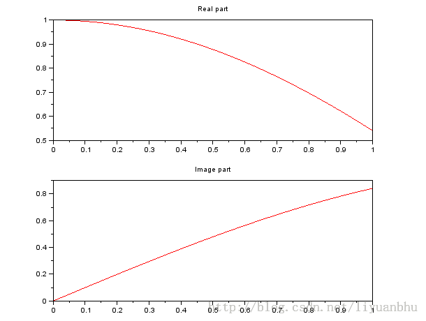
~~~
t = linspace(0,1,101);
y1 = exp(%i*t);
subplot(2,1,1);
plot(t,real(y1),'r');
xtitle("Real part");
subplot(2,1,2);
plot(t,imag(y1),'r');
xtitle("Image part");
~~~
另一种常见的需求是我们希望同时能有多个图形窗口,每个窗口绘制不同的内容。
这时可以用 scf() 函数。
Scf 函数有三种基本的调用形式:
f = scf()
f = scf(h)
f = scf(num)
第一种方式不输入任何参数,这时scilab 自动生成一个新的空白窗口。然后我们就可以在这个空白窗口上绘图了。返回值是这个窗口的句柄,利用这个句柄可以设置这个窗口的各种属性。
第二种方式将句柄为h 的窗口设置为当前窗口,之后任何的绘图动作都是在这个窗口中操作的。
第三种是将窗口号为num的窗口设为当前窗口,如果没有这个窗口则新建一个。
如果我们想将某个窗口的内容清空,可以使用函数 clf(),它也有三种基本调用方法。
clf()
clf(h)
clf(num)
第一种是清空当前窗口。第二种是清空句柄为h 的窗口,第三种是清空窗口号为num 的窗口,第三个是清空窗口号为num的窗口。
下面是个非常简单的例子:
~~~
x = linspace(0, 2*%pi, 101);
scf(1);
clf(1);
plot(x,sin);
scf(2);
clf(2);
plot(x,cos);
~~~
Scilab 的绘图函数(3)
最后更新于:2022-04-01 07:32:15
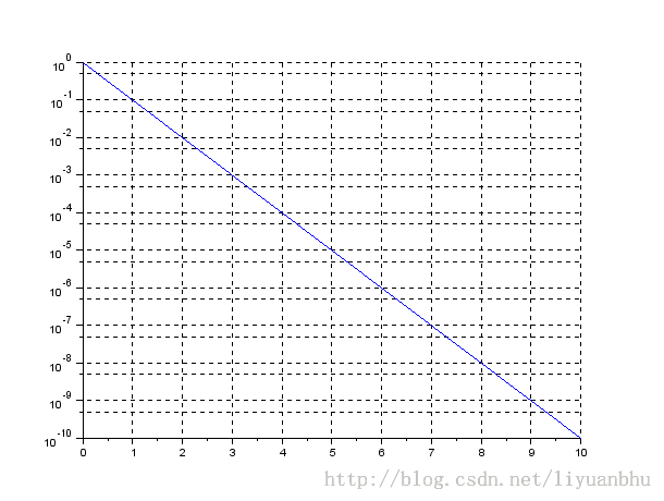
我们在做数据绘图或函数图像时经常需要使用对数坐标系。尤其是数据的范围跨越很多个数量级时,通常的线性坐标系下无法表现出数据特征。
Scilab 中Plot函数无法画出对数坐标。需要使用 plot2d 函数。
plot2d 函数的基本用法如下:
plot2d([logflag,][x,],y[,style[,strf[,leg[,rect[,nax]]]]])
plot2d([logflag,][x,],y,<opt_args>)
下面是一个简单的例子:
~~~
iter = linspace(0,10,11);
err = 10.^(-iter);
plot2d("nl", iter, err, style=2);
set(gca(),"grid",[1 1]);
~~~
这个例子如果在普通的坐标系下看,是这个样子的:
~~~
plot(iter,err);
set(gca(),"grid",[1 1]);
~~~
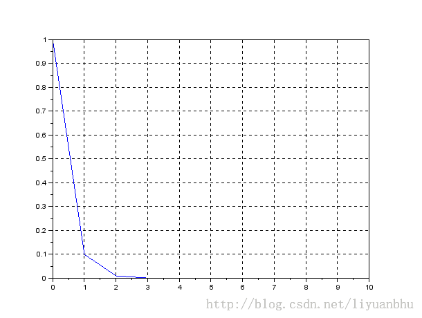
由于数据很快就很接近0了,在图中很难看出后面的趋势。
下面来详细的讲解一下plot2d函数。
plot2d("nl", iter, err, style=2);
“nl” 表示,横坐标为正常的模式(normal),纵坐标为对数(log).
Style = 2 表示的是曲线的颜色。2 表示的是colormap 中的第二项,也就是蓝色。
如果是负数,则表示用不同的线型。如果既要设置曲线的颜色,又要设置线型,那么。。。暂时还没搞定。
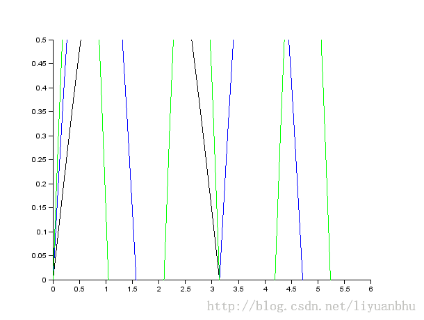
下面再给一个例子,通过rect参数控制xy的范围:
~~~
x=[0:0.1:2*%pi]';
plot2d(x,[sin(x) sin(2*x) sin(3*x)],rect=[0,0,6,0.5]);
~~~
有点跑题了,接着介绍对数坐标系绘图。下面再给一个例子:
~~~
ind = linspace(0,6,7);
iter = 10.^ind;
err1 = 10.^(-ind);
err2 = (10.^(-ind)).^2;
xset("font size", 4);
plot2d("ll", iter, err1, style=2);
plot2d("ll", iter, err2, style=3);
title("Loglog","fontsize", 4);
xlabel("Iterations","fontsize", 4);
ylabel("Error","fontsize", 4);
set(gca(),"grid",[5 5]);
legend(['error1';'error2'],"in_lower_left");
~~~
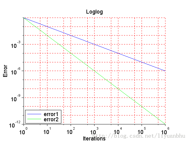
这个图是双对数坐标,同时还调整了图上的文字。需要注意的是:
xset("font size", 4);
语句一定要在
legend(['error1';'error2'],"in_lower_left");
语句之前调用,否则得到的图形的legend 的字号会有问题,下面是个实验,先执行如下语句:
~~~
ind = linspace(0,6,7);
iter = 10.^ind;
err1 = 10.^(-ind);
err2 = (10.^(-ind)).^2;
plot2d("ll", iter, err1, style=2);
plot2d("ll", iter, err2, style=3);
title("Loglog","fontsize", 4);
xlabel("Iterations","fontsize", 4);
ylabel("Error","fontsize", 4);
set(gca(),"grid",[5 5]);
legend(['error1';'error2'],"in_lower_left");
~~~
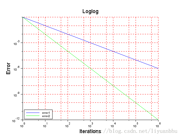
这个图形是和我们的预期一样的。标题和Label的字号变大了,刻度和Legend的字号还是原来的大小。
接着执行:
~~~
xset("font size", 4);
~~~
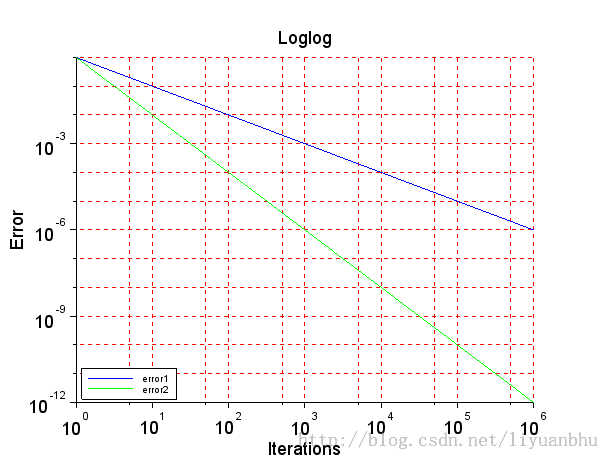
结果是刻度上的字号更新为正确的大小了,可legend 的字号没变。看来这个是 scilab 的一个bug。
所以我们需要先设置字号,然后调用legend 函数。
Scilab 的绘图函数(2)
最后更新于:2022-04-01 07:32:13
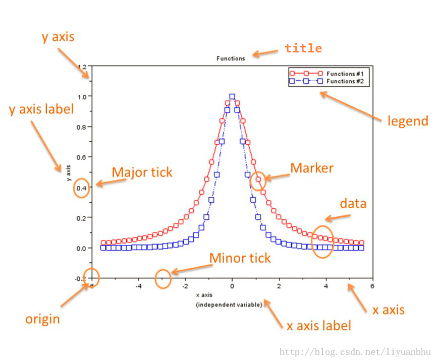
一幅图是由许多元素组成的。包括图标题,x轴标签,y轴标签,刻度线等。图1给出了各个元素的一个示意图。
这些所有的元素在scilab中都是可以用代码控制的。
### 标题
上个笔记上介绍了用xtitle()函数可以在图上添加标题。比如:
~~~
title("My Plot");
~~~
实际上,title函数有三种形式:
title(my_title)
title(my_title,<Property>)
title(<axes_handle>,<my_title>,<Property>)
上次只是用的最简单的形式,利用第二种形式就可以设置标题的字体、字号等属性了。下面给个例子:
~~~
x = 0:0.1:10;
plot(x, sin);
title("$f=sin(x)$","fontname","helvetica bold", "fontsize", 4, "color", "red");
~~~
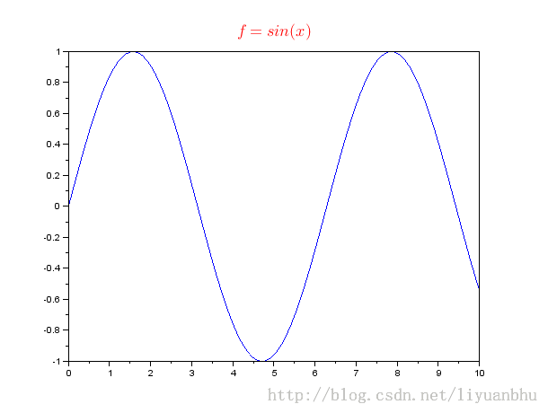
上面例子中,"$f=sin(x)$" 是 Latex 代码片段,scilab 支持基本的latex 数学模式,因此可以产生漂亮的标题。
后面设置了字体为helvetica bold, 字号大小为4,颜色为红色。除此之外还可以设置其他的参数,具体可以参阅帮助文档。
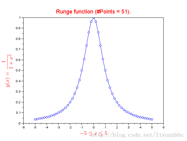
X 轴的Label 和y轴的Label 有两个独立的函数来设置。这两个函数的用法与 title 函数基本相同,下面举个例子:
~~~
x = linspace(-5,5,51);
y = 1 ./(1+x.^2);
plot(x,y,'o-b');
xlabel("$-5\le x\le 5$","fontsize",4,"color","red");
ylabel("$y(x)=\frac{1}{1+x^2}$","fontsize",4,"color","red");
title("Runge function (#Points ="+string(length(x))+").","color","red","fontsize",4);
~~~
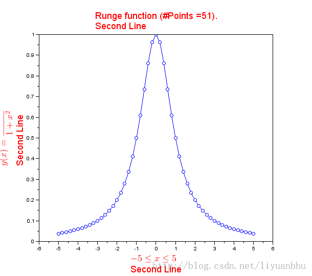
另外,无论是标题还是Label,都可以是多行的,对上面的例子稍作修改。
~~~
xlabel(["$-5\le x\le 5$";"Second Line"],"fontsize",4,"color","red");
ylabel(["$y(x)=\frac{1}{1+x^2}$";"Second Line"],"fontsize",4,"color","red");
title(["Runge function (#Points ="+string(length(x))+").";"Second Line"],"color","red","fontsize",4);
~~~
如果有多条曲线,就需要有个legend 来说明哪条曲线是什么。见下面的例子:
~~~
x = linspace(-5.5,5.5,51);
y = 1 ./(1+x.^2);
plot(x,y,'ro-');
plot(x,y.^2,'bs:');
xlabel(["x axis";"(independent variable)"],"fontsize", 4);
ylabel("y axis","fontsize", 4);
title("Functions","fontsize", 4);
legend(["Functions #1";"Functions #2"])
~~~
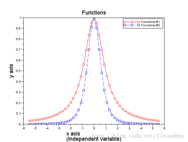
Legend 的字体和字号不能像label 那样设置。实验后发现,legend 和刻度上的字共用一套控制命令:
~~~
xset("font size", 4);
~~~
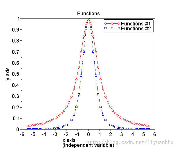
至此,这幅图就比较漂亮了。
下次讲讲如何在对数坐标系下绘图。未完待续!
Scilab 的绘图函数(1)
最后更新于:2022-04-01 07:32:09
# Scilab 的绘图函数
### plot 函数
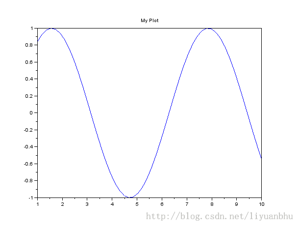
最基本的是 plot 函数,与 matlab 中的plot 函数类似。
~~~
xdata = linspace(1,10,50);
ydata = sin(xdata);
plot(xdata, ydata);
~~~

对函数绘图,不需要事先计算出 ydata,比如下面的例子画出的结果是相同的。
~~~
plot (xdata, sin);
~~~

这样还能节省些内存占用。
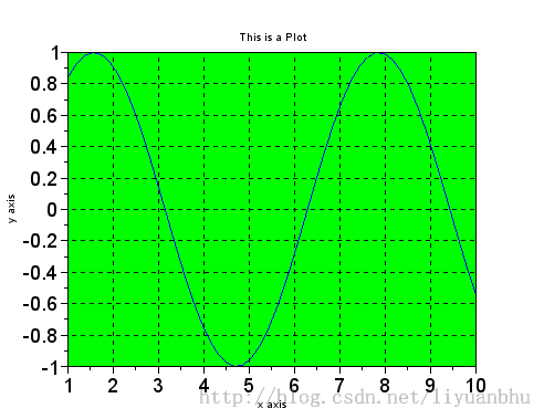
如果只设置总的标题,可以这样操作:
~~~
title("My Plot");
~~~
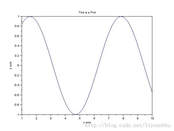
如果还要设置XY坐标轴的标题,那么可以这样:
~~~
xtitle("This is a Plot", "x axis", "y axis");
~~~
颜色和线型可以通过给plot 添加第三个参数来控制。Legend() 函数可以设置标签。比如下面的例子:
~~~
plot(xdata, sin, "o-r");
plot(xdata, cos, "*--y");
legend("sin", "cos");
~~~
### 保存图片
一幅图绘制完成之后当然希望能够保存到文件中,scilab 支持相当多的图片格式,下面这些函数每个对应一种图片格式。
<table height="169" width="268"><tbody><tr><td valign="top"><p>xs2png</p></td><td valign="top"><p>xs2fig</p></td></tr><tr><td valign="top"><p>xs2pdf</p></td><td valign="top"><p>xs2gif</p></td></tr><tr><td valign="top"><p>xs2svg</p></td><td valign="top"><p>xs2jpg</p></td></tr><tr><td valign="top"><p>xs2ps</p></td><td valign="top"><p>xs2bmp</p></td></tr><tr><td valign="top"><p>xs2emf</p></td><td valign="top"><p>xs2ppm</p></td></tr></tbody></table>
如果我们希望将 0 号窗口的图形保存为png 格式,那么可以执行下面的语句。
~~~
xs2png(0, "pic.png");
~~~
上面提到了窗口号,在绘图窗口上写着这个数字。Scilab 同时可以显示多个图像窗口,通过窗口号来区分现在操作的是哪个绘图窗口。
很多时候我们希望能够在图像上添加网格,这个操作在MATLAB很容易实现:
Grid on 开启网格
Grid off 关闭网格
Scilab 中没有这样的语句,但是可以用如下的语句来代替。
开启网格:
~~~
set(gca(),"grid",[1 1]);
~~~
关闭网格:
~~~
set(gca(),"auto_clear",[-1 -1]);
~~~
下面是开启网格之后的效果:
设置坐标轴上刻度的字的大小:
~~~
xset("font size", 4);
~~~
很悲催,这样设置对标题的字号无效。。。还没有解决办法。
设置图片的背景色:
~~~
xset("background", color);
~~~
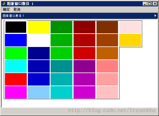
其中 color 为一个整数,表示的是colormap 中的索引。可以用 getcolor() 函数获得当前的colormap。
~~~
getcolor();
~~~
将背景色设置为绿色
~~~
xset("background", 3);
~~~
(未完待续)
利用 SCILAB 设计 iir 滤波器设计(模拟滤波器双线性变换法)
最后更新于:2022-04-01 07:32:04
IIR 滤波器的设计方法有很多种,一种比较简单的方法是先设计对应的模拟滤波器,然后将模拟滤波器转换为对应的数字滤波器。模拟滤波器到数字滤波器的转换最常见的方法是双线性变换法。下面就介绍一下怎么利用SCILAB提供的函数利用这种方法设计一个IIR 滤波器。
hz=iir(n,ftype,fdesign,frq,delta)
[p,z,g]=iir(n,ftype,fdesign,frq,delta)
Arguments
N : 滤波器的阶数
Ftype 滤波器的类型,’lp’ 表示低通,'hp' 表示高通,'bp' 表示带通,'sb' 表示带阻。
Fdesign:指定模拟滤波器的类型,可以为 'butt', 'cheb1', 'cheb2' ,'ellip'
Frq: 长度为2的向量,指定滤波器的截止频率,这里的频率为归一化的频率,采样频率归一化为1。对于低通和高通滤波器,只有第一个参数有用,带通和带阻滤波器这两个截止频率都要用到。
Delta:长度为2的向量,对于cheb1型滤波器,只有第一个参数有用, 对于cheb2 型滤波器,只用到第二个参数,ellip 滤波器这两个参数都用到了 0<delta(1),delta(2)<1
对cheb1 型滤波器:1-delta(1)<ripple<1 ,限定了通带的波动
对cheb2 型滤波器: 0<ripple<delta(2) ,限定了阻带的波动
对ellip 型滤波器:
在通带,1-delta(1)<ripple<1
在阻带,0<ripple<delta(2)
Hz:计算出的系统函数
P:给出了滤波器的各个零点
z:给出了滤波器的各个极点
G:增益
下面给个具体的例子:
hz=iir(3,'bp','ellip',[.15 .25],[.08 .03]);
这个例子设计的是一个 3 阶带通椭圆滤波器。通带截止频率为 0.15 和 0.25,通带允许波动为 0.08, 阻带允许波动为 0.03。
计算出的滤波器传递函数为:
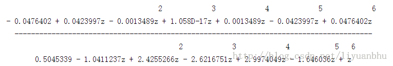
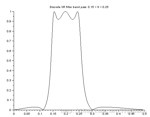
下面画出频响曲线:
[hzm,fr]=frmag(hz,256);
plot2d(fr',hzm')
xtitle('Discrete IIR filter band pass 0.15 < fr < 0.25 ',' ',' ');
如果我们需要零极点信息的话,可以这样计算:
[p,z,g]=iir(3,'bp','ellip',[.15 .25],[.08 .03]);
Z 给出的是零点的位置,q是极点位置:
z =
0.7632657 + 0.6460848i
0.7632657 - 0.6460848i
1.
- 0.3182662 - 0.9480014i
- 0.3182662 + 0.9480014i
- 1.
p =
0.5561319 - 0.7583880i
0.5561319 + 0.7583880i
0.2703756 + 0.7688681i
- 0.0034896 + 0.9267011i
- 0.0034896 - 0.9267011i
0.2703756 - 0.7688681i
利用 SCILAB 设计 FIR 滤波器(Minimax法)
最后更新于:2022-04-01 07:32:02
所谓 Minimax 方法就是指设计的指定阶数的FIR滤波器的幅度响应的最大偏离最小化。SCILAB 提供了eqfir 函数可以方便的使用 minmax 法设计FIR 滤波器。
[hn]=eqfir(nf,bedge,des,wate)
其中:
Nf: FIR 滤波器的阶数
Bedge: M * 2 的矩阵,矩阵的每一行对应一个频率段
Des: M 个元素的向量,每个元素给出一个频率段的期望的幅度响应
Wate: M 个元素的向量,给出每个频率段的加权系数
返回值:
Hn: FIR 滤波器的系数
下面给个例子:
hn=eqfir(33,[0 0.2;0.25 0.35;0.4 0.5],[0 1 0],[1 1 1]);
这个例子是设计一个 33 阶的FIR 滤波器, [0 0.2] 这一频段的期望幅度为0,[0.25 0.35] 这一频段的期望幅度为1,[0.4 0.5] 这一段的期望幅度为 0。没有给出的频段为过渡段,幅度为多少都可以。
可以用 frmag 函数来观测上面设计的滤波器的频率响应。
[xm,fr]=frmag(num,den,npts)
Num 为系统函数的分子。也就是我们FIR滤波器的系数。
Den 为系统函数的分母,对于FIR滤波器来说,分母为1。
Npts 为频率响应的数据点数
返回值;
Fr 为频率点
Xm 为对于的频率响应
对于上面的例子,我们可以写:
[xm,fr]=frmag(hn,1,100);
plot(fr,xm);
利用 SCILAB 设计 FIR 滤波器(窗函数法)
最后更新于:2022-04-01 07:32:00
理论上说,设计FIR滤波器是很简单的,给定一个期望的频率响应H(ω),对其进行傅里叶反变换就可以得到FIR滤波器的离散单位冲击响应。
实际使用中的问题是,这样得到的许多滤波器的滤波器阶数都是无穷的而且得到的滤波器不一定是因果系统。
比如理想低通滤波器,截止频率为ωc
计算得到的滤波器系数为:
一种简单的办法是将这个序列中间的一部分截取出来。也就是对信号加一个矩形的窗函数。
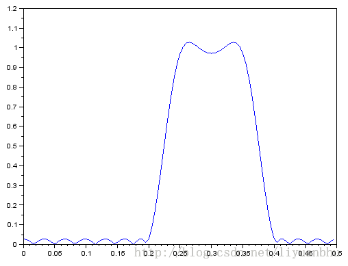
当N = 33 截止频率ωc =0.2时滤波器的频率响应如下图所示,其中实线是理想低通滤波器的响应曲线。加窗的结果是频响曲线在通频带和阻带都产生了波动,偏离理想低通滤波器频响曲线最大的地方在ωc处。
除了用矩形窗函数,还可以采用其他形状的窗函数,不同类型的窗函数有不同的特点。关于不同窗函数的特征请参见数字信号处理方面的教材,这里不多说了。
### wfir
[wft,wfm,fr]=wfir(ftype,forder,cfreq,wtype,fpar)
Ftype 表示滤波器的类型,可以为'lp','hp','bp','sb'
Forder 为滤波器的阶数
Cfreq 为滤波器的转折频率,对于低通和高通滤波器来说提供一个截止频率就行了,对于带通和带阻滤波器要提供2个转折频率。这里的频率都是归一化了的,采样频率被归一化为1。
所以转折频率要小于 0.5。
Wtype 表示窗函数的类型,可以为 're','tr','hm','hn','kr','ch'
Fpar 表示窗函数的参数,长度为2的数组,只对 Kaiser 窗 和Chebyshev 窗有效。
对 Kaiser 窗fpar(1)>0, fpar(2)=0.
对Chebyshev 窗fpar(1)>0, fpar(2)<0 或者 fpar(1)<0, 0<fpar(2)<.5
返回值:
Wft 为返回的滤波器系数
Wfm 为滤波器的频响特性
Fr 为Wfm 对应的频率点
下面举一个具体的例子:
[h,hm,fr]=wfir("lp",33,[.2 0],"hm",[0 0]);
这个表示低通滤波器,33阶,截止频率0.2,hamming 窗
Plot(fr,hm);
窗函数法设计FIR滤波器器介绍这些也就差多不了,下次介绍频率抽样法。
Scilab 处理声音数据(补充)
最后更新于:2022-04-01 07:31:57
### mapsound
Scilab 中有一个函数可以绘制声音频谱随时间变化的图像。采用的算法是分块进行FFT求得每一时间段内的频谱。唯一一点缺陷是窗函数无法选择,只能是矩形窗。算是个简化版本的短时傅里叶变换。
mapsound (w,dt,fmin,fmax,simpl,rate)
其中 w 是声音数据
Dt 是时窗的宽度,单位是秒
Fmin 和Fmax 限定了绘制的图像的y轴的最小和最大值,单位 Hz。
Simpl 表示在计算时将多少个相邻数据点合成一个数据点计算。
Rate 是信号的采样率
以上各参数的默认值如下:
Dt: 0.1
Fmin: 100
Fmax: 1500
Simpl :1
Rate: 22050
~~~
// At first we create 0.5 seconds of sound parameters.
t=soundsec(0.5);
// Then we generate the sound.
s=sin(440*t)+sin(220*t)/2+sin(880*t)/2;
[nr,nc]=size(t);
s(nc/2:nc)=sin(330*t(nc/2:nc));
mapsound(s,0.1,100,500,1);
~~~
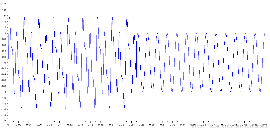
原始声音数据的波形如下:
上面例子中用到了另一个函数soundsec,这个函数的作用很简单,生成一个 n 秒声音数据所需的时间向量。
t=soundsec(n [,rate])
N 是要生成的声音数据的时长
Rate 采样率
scilab 读取处理 wav 文件 (2)
最后更新于:2022-04-01 07:31:55
上一篇 blog 中已经介绍了 wavread 和 wavwrite 两个函数。这里介绍其他一些有用的函数。
###
playsnd 函数
播放声音数据。基本用法如下。 其中 command 只在 unix 类系统中用到。用来指定播放声音的程序。 Win 下无需考虑。
[]=playsnd(y)
[]=playsnd(y,rate,bits [,command])
如果不指定 rate 则默认是 22050
Bits 在当前版本中其实没有用,所以无需设置。
我通常会用高采样率采集声音,然后在这里设个低的 rate,将声音慢放出来。细节就可以听的很清楚了。
###
Sound 函数
Sound 函数的作用和 Playsnd 函数完全相同。不知道scilab 为什么要将这两个函数都保留了下来。
sound(y [,fs,bits,command)
###
Auread 函数
读取 .au 文件,用法基本和 wavread 是相同的。下面使用法举例,各个参数的含义与 wavread 中对应参数相同。因此这里就不多解释了。
y=auread(aufile)
y=auread(aufile,ext)
[y,Fs,bits]=auread(aufile)
[y,Fs,bits]=auread(aufile,ext)
###
Auwrite 函数
将数据写到一个 .au 文件中。
auwrite(y,aufile)
auwrite(y,Fs,aufile)
auwrite(y,Fs,bits,aufile)
auwrite(y,Fs,bits,method,aufile)
###
Analyze 函数
绘制声音数据的频谱图。
analyze(y, fmin, fmax, fs, points);
下面举个例子
[y,fs,bits]=wavread("C63A 4331440.wav");
Plot(y);
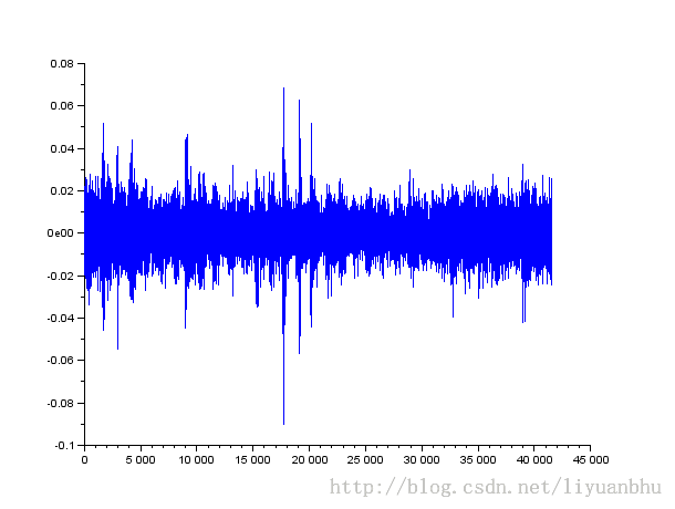
analyze(y, 100, 15000, fs, size(y,2));
scilab 读取处理 wav 文件
最后更新于:2022-04-01 07:31:53
最近工作需要,要对wav文件中存储的声音信息进行分析处理。所以花了些时间收集了各种数学软件中处理wav 文件的方法。
### Scilab
Scilab 中处理音频文件的函数很多。其中最基本的是wavread和wavwrite。
~~~
y=wavread(wavfile)
~~~
将wav 文件中的波形数据读入 y 中,波形的幅度范围在[-1, 1]。与Matlab 不同,scilab 将波形数据存成行向量而不是列向量。
~~~
[y,Fs,bits]=wavread(wavfile)
~~~
Fs 存的是采样率,单位Hz,bits 是数据的位数。
~~~
wavread(wavfile,n)
~~~
读取波形文件的前n个数据点。
~~~
wavread(wavfile,[n1,n2])
~~~
只读取n1 到 n2 之间的数据。
~~~
siz = wavread(wavfile,'size')
~~~
读取wav文件有多少数据点,siz 为一个1行两列的向量。siz = [channels samples] 这里与Matlab 返回的结果也正好是相反的。
~~~
wavread(wavfile,'info')
~~~
读取wav 文件的信息,返回一个行向量 [数据类型,通道数, 采样率, 每秒需要多少个字节, byte alignment of a basic sample block, 数据的位数, 每个数据点占的字节数, 每通道的字节数].
~~~
wavwrite(y, wavfile)
~~~
将 y 中的数据写入 wavfile 中,采样率默认为 22500 Hz, 16 bits。
~~~
wavwrite(y, Fs, wavfile)
~~~
Fs 用来设定采样率。
~~~
wavwrite(y, Fs, nbits, wavfile)
~~~
nbits指定数据的位数,可以为 8、16、24和32。当 nbits!=32时,wav文件按照PCM 码来存储。当nbits=32时,数据按照浮点数格式存储。这时也就不要求数据范围在-1到1 之间了。
另一个类似作用的函数如下:
~~~
savewave(filename,x [, rate , nbits]);
~~~
gnuplot 读取逗号分隔的数据文件
最后更新于:2022-04-01 07:31:51
有时,我们的数据文件中各个数据之间是用逗号作为分隔符的,比如标准的以“CSV”为后缀的那种数据文件。如果在逗号之后没有空格分隔,默认情况下gnuplot是无法直接读取的。
这时可以有两种方案,第一种是提前处理一下数据文件,比如将逗号替换为空格,随便一个文本处理软件都能很轻松的做这种替换。但是有时我们有很多这样的数据文件,每个都这样处理一下也挺麻烦的。
第二种方法就是在gnuplot中给出文件分隔符的信息,让gnuplot能够读懂我们的文件。下面将要说的就是这种方法。
比如我们有如下的文件:
~~~
-3,0.1,0.0001234098
-2.9,0.1062699256,0.0002226299
-2.8,0.1131221719,0.000393669
-2.7,0.1206272618,0.0006823281
-2.6,0.1288659794,0.0011592292
-2.5,0.1379310345,0.0019304541
-2.4,0.1479289941,0.0031511116
-2.3,0.1589825119,0.0050417603
-2.2,0.1712328767,0.0079070541
-2.1,0.1848428835,0.0121551783
-2,0.2,0.0183156389
-1.9,0.2169197397,0.0270518469
-1.8,0.2358490566,0.0391638951
-1.7,0.2570694087,0.0555762126
-1.6,0.2808988764,0.0773047404
-1.5,0.3076923077,0.1053992246
-1.4,0.3378378378,0.1408584209
-1.3,0.3717472119,0.184519524
-1.2,0.4098360656,0.2369277587
-1.1,0.4524886878,0.2981972794
-1,0.5,0.3678794412
-0.9,0.5524861878,0.4448580662
-0.8,0.6097560976,0.527292424
-0.7,0.6711409396,0.6126263942
-0.6,0.7352941176,0.6976763261
-0.5,0.8,0.7788007831
-0.4,0.8620689655,0.852143789
-0.3,0.9174311927,0.9139311853
-0.2,0.9615384615,0.9607894392
-0.1,0.9900990099,0.9900498337
0,1,1
0.1,0.9900990099,0.9900498337
0.2,0.9615384615,0.9607894392
0.3,0.9174311927,0.9139311853
0.4,0.8620689655,0.852143789
0.5,0.8,0.7788007831
0.6,0.7352941176,0.6976763261
0.7,0.6711409396,0.6126263942
0.8,0.6097560976,0.527292424
0.9,0.5524861878,0.4448580662
1,0.5,0.3678794412
1.1,0.4524886878,0.2981972794
1.2,0.4098360656,0.2369277587
1.3,0.3717472119,0.184519524
1.4,0.3378378378,0.1408584209
1.5,0.3076923077,0.1053992246
1.6,0.2808988764,0.0773047404
1.7,0.2570694087,0.0555762126
1.8,0.2358490566,0.0391638951
1.9,0.2169197397,0.0270518469
2,0.2,0.0183156389
2.1,0.1848428835,0.0121551783
2.2,0.1712328767,0.0079070541
2.3,0.1589825119,0.0050417603
2.4,0.1479289941,0.0031511116
2.5,0.1379310345,0.0019304541
2.6,0.1288659794,0.0011592292
2.7,0.1206272618,0.0006823281
2.8,0.1131221719,0.000393669
2.9,0.1062699256,0.0002226299
3,0.1,0.0001234098
~~~
可以看到,数据有三列,用逗号来分隔,我们下面的例子中之用到前两列。如果直接用如下命令的话得到的不是我们希望的结果。
~~~
Plot 'sample.csv'
~~~
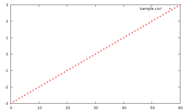
gnuplot 只解析出了第一列的数据。如果我们告诉gnuplot我们的数据有两列会怎样呢?
~~~
Plot 'sample.csv' using 1:2
~~~
gnuplot 会抱怨说:
~~~
gnuplot> plot 'sample.csv' using 1:2
^
warning: Skipping data file with no valid points
^
x range is invalid
~~~
正确的方法是这样的:
plot 'sample.csv' using 1:2 "%lf,%lf"
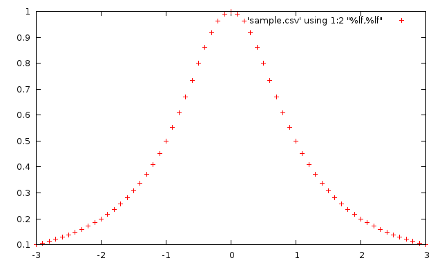
格式字符串的格式与C语言中scanf的格式字符串是类似的,实际上gnuplot最后就是用的scanf函数来读取数据。%lf表示按照 double型浮点数类型来读取。需要注意的是gnuplot的格式化字符串不支持%f。
gnuplot的格式化字符串还有很多的用法,这里就不多介绍了,有兴趣的可以参考帮助文档相关章节。
gnuplot 入门教程 4
最后更新于:2022-04-01 07:31:48
# 绘图环境参数
如第二章所述,只要键入 plot sin(x), '1.dat' 即可得到图1 的结果。gnuplot 自动调整 X 轴、 Y 轴的显示范围,使图形显示在适当的位置并选择不同的颜色、图形,用以区别不同的函数或数据,也就是 gnuplot 自动调整其所需的绘图环境。若我们需要一些特别的绘图参数,如在 3D 中加入等高线、设定消去隐藏线、改变 X 轴、Y 轴的座标点名称等,可由改变绘图环境参数而改变之。 本章说明这些绘图参数设定的方法与功能。
### Axis
绘图参数在设定坐标轴方面的参数可分为变量名称、数字格式、网格、显示范围、坐标轴显示方式与显示与否等六方面的设定:
### 变量名称设定
一般以 x 为横轴上的变量。可用 dummy 设定为其它的名称, 所绘函数的变量名称亦随之改变。如 set dummy t 将自变量改为 t,图8、图17、图20 均改变自变量名称。
### 数字格式设定
设定数字的显示方式与格式。由 format 此项参数设定显示格式,其语法为 :
~~~
set format {<axes>} {"<format-string>"}
show format # 显示各轴数字显示的型式
~~~
其中 axis 为 x、y、z、xy 或预设为xy。format-string 为描述数字格式的字符串,可接受如 C 语言中 printf 对数字的 f、e、g 三种格式化描述,亦可加入文字 (必须少于100 字)。以下举一些例子:
~~~
set format xy "%.2e"
set format x "%3.0f cm"
~~~
显示方式由 tics、xtics等设定。
xtics 是对 X 坐标轴上的格点做设定。如起始点、结束点、间隔或在轴上特定点放特定的名称。其语法为:
~~~
set xtics { {<start>, <incr>{, <end>}} |
{({"<label>"} <pos> {, {"<label>"} <pos>}...)} }
set noxtics # 不标示任何 X 轴上的标点。
show xtics # 显示 X 轴标点的状况。
~~~
下面是三个改变格点的例子。
~~~
# 每隔 2 格一个标点
set xtics -10,2,10
plot sin(x)
~~~

~~~
# 以文字作为标点
set xtics ("low" -10, "medium" 0, "high" 10)
plot sin(x)
~~~

~~~
# 在特定位置放上标点
set xtics (-10,-9,-7,-3,0,pi/2,2*pi)
plot sin(x)
~~~

xdtics 将 X 座标轴上标点名称依 0,1,…改为 Sun,Mon,… Sat 等。 大于 7 的数目除以7 取其馀数。
~~~
# 将标点名称改为 Sun, Mon, ... Sat 等
set xdtics
plot [0 : 10] sin(x)
~~~

ytics, ymtics, ydtics, ztics, zmtics, zdtics 与 xtics, xmtics, xdtics 相似,不同点是作用在不同的轴上。
ticslevel 是在画 3D 图形时,调整 Z 轴的相对高度。语法为:
~~~
set ticslevel {<level>}
show tics
~~~
### 网格设定
在 XY 座标平面上依刻度画上方格子。
~~~
# 设定变数为 t
set dummy t
# 设定 X 轴 Y 轴标点的格式
set format xy "%3.2f"
# 产生网格
set grid
plot sin(t)
~~~

### 座标显示方式
分为线性与对数两种。一般为前者,若要改为对数方式,其语法为:
~~~
set logscale <axes> <base>
set nologscale <axes>
show logscale
~~~
其中 axes 为 X 轴、Y 轴、Z 轴的任意组合。base 预设为 10。
### 显示范围设定
改变各轴的显示范围。autoscale 参数设定后 gnuplot 自动调整显示范围。其余的如 rrange, trange, xrange, yrange, zrange 则是由使用者设定该轴的范围,以 xrange 为例,其语法为:
~~~
set xrange [{<xmin> : <xmax>}]
~~~
其中参数 <xmin> 与 <xmax> 代表 X 轴的起点与终点, 可以是数字或数学式子。如图7 中 set [0:10] sin(x) 设定 X 轴显示范围为 0 与 10 之间。此时可用
~~~
set xrange [0:10]
plot sin(x)
~~~
使用 autoscale 参数调整显示范围,其语法为:
~~~
set autoscale <axes>
set noautoscal <axes>
show autoscale
~~~
其中 <axes> 为 gnuplot 欲调整的轴,可以是 x, y, z 或 xy,预设为所有的轴。
### 座标轴显示与否设定
设定是否要画出座标轴,以 X 轴为例:
~~~
set xzeroaxis # 设定显示 X 座标轴
set noxzeroaxis # 设定不显示 X 座标轴
show xzeroaxis # 检查 X 座标轴显示与否
~~~
### Label
gnuplot 除了绘出图形外,尚可加入注解做为辅助说明。这注解包括文字与线条两方面,其提供的设定有:
<table><tbody><tr><td valign="top"><p>功能</p></td><td valign="top"><p>绘图参数名称</p></td></tr><tr><td valign="top"><p>线条</p></td><td valign="top"><p>arrow</p></td></tr><tr><td valign="top"><p>文字注解</p></td><td valign="top"><p>key, label, time, title, xlabel, ylabel, zlabel</p></td></tr></tbody></table>
### 线条
在图上画一线段可以选择有无箭头。其语法为:
~~~
set arrow {<tag>} {from <sx>,<sy>{,<sz>}}
{to <ex>,<ey>{,<ez>}} {{no}head}
unset arrow {<tag>} # 删除一线条
show arrow # 显示线条使用情况
~~~
其中参数 <tag> 是给该条线条一个整数名称,若不设定则为最小可用整数。此线条由坐标 (sx, sy, sz) 到 (ex, ey, ez) (在 2D 中为 (sx, sy)到(ex, ey))。参数 nohead 为画没有箭头的线段,参数 head 或没有 nohead 为画有箭头的线段。图24 中使用没有箭头的线段作为辅助说明。以下为一些例子:
~~~
# 画一带有箭头的线条由原点到 (1,2)。
set arrow to 1,2
# 画一名为 3 的带箭头线条 由 (-10,4,2) 到 (-5,5,3)。
set arrow 3 from -10,4,2 to -5,5,3
# 改变名为 3 的线条起始点至 (1,1,1)。
set arrow 3 from 1,1,1
# 删除名为 2 的线条。
unset arrow 2
# 删除所有线条。
unset arrow
# 显示线条的使用情形。
show arrow
~~~
### 文字注解
分为设定标题 (title),标示 (label) 与时间 (time) 三部份。标题设定为在图的正上方加上说明本图的文字。其语法为:
~~~
set title {"<title-text>"} {<xoff>}{,<yoff>}
show title
~~~
设定参数 <xoff> 或 <yoff> 为微调标头放置的位址。 xlabel, ylabel, zlabel 的语法与 title 相同,其各自描述一坐标轴。
标示 (label) 为在图上任一位置加上文字说明,一般与线条一并使用。其语法为:
~~~
set label {<tag>} {"<label_text>"}
{at <x>,<y>{,<z>}}{<justification>}
unset label {<tag>} # 删除一标示
show label # 显示标示使用情况
~~~
其中参数 <tag> 与 "线条" (arrow) 中 <tag> 意义相同,用以区别不同的 label。参数 <justification> 是调整文字放置的位置,可以是 left,right 或 center。举一些例子:
~~~
# 将 y=x 放在座标 (1,2) 之处。
set label "y=x" at 1,2
# 将 y=x^2 放在座标 (2,3,4) 之处,并命名为 3。
set label 3 "y=x^2" at 2,3,4 right
# 将名为 3 的标示居中放置。
set label 3 center
# 删除名为 2 的标示。
set nolabel 2
# 删除所有标示。
set nolabel
# 显示标示使用情形。
show label
~~~
一般绘一图形后,gnuplot 将函数名称或图形名称置于右上角。 key 参数设定可改变名称放置位置。其语法为:
~~~
set key
set key <x>,<y>{,<z>}
unset key
show key
~~~
其中参数 <x>, <y>, <z> 设定名称放置位置 。unset key 为不显示名称,若使用 set key 则再度显示名称。若使用 set key 0.2, 0.5 则显示函数名称于坐标 (0.2, 0.5) 之处。
~~~
unset key
plot sin(x), cos(atan(x))
~~~

~~~
set key at 2, 0.5
plot [-pi/2:pi] cos(x), -( sin(x) > sin(x+1) ? sin(x) : sin(x+1))
~~~

时间参数设定是将图产生的时间标在图上。其语法为
~~~
set time {<xoff>}{,<yoff>}
unset time
show time
~~~
设定参数 <xoff> 或 <yoff> 为微调时间放置的位址,正数表示向上或向右,负数为反方向,以字的长宽作为单位。
~~~
set title "sin(x)+sin(2*x)"
set xlabel "X-axis"
set ylabel "Y-axis"
set arrow from -2,1 to -2.5,0.4
set label "Local max" at -2,1.1
unset key
set time
plot [-5:5] sin(x)+sin(2*x)
~~~

gnuplot 入门教程 3
最后更新于:2022-04-01 07:31:46
# 常量、操作符和函数
### 数字
gnuplot 表示数字可分成整数、实数及复数三类:
整数:gnuplot 与 C 语言相同,采用 4 byte 储存整数。故能表示 -2147483647 至 +2147483647 之间的整数。
实数:能表示约 6 或 7 位的有效位数,指数部份为不大于 308 的数字。
复数:以 {<real>,<imag>} 表示复数。其中<real>为复数的实数部分,<imag>为虚数部分,此两部分均以实数型态表示。 如 3 + 2i 即以 {3,2} 表示。
gnuplot 储存数字的原则为,若能以整数方式储存则以整数储存数字,不然以实数方式储存,其次以复数方式储存。例如在 gnuplot 执行
~~~
print 1/3*3
print 1./3*3
~~~
分别得到 0 和 1.0 的结果。这是因前者使用整数计算,而后者采用实数计算的结果。执行
~~~
print 1234.567
print 12345 + 0.56789
print 1.23e300 * 2e6
print 1.23e300 * 2e8
~~~
分别得到 1234.57、12345.6、2.46e+304 和 undefined value 的结果。这些例子是受到实数的有效位数和所能表现最大数字的限制。这是我们要注意的。
### 操作符
gnuplot 的操作符与 C 语言基本相同。 所有的操作均可做用在整数、实数或复数上。
表格 1 Unary Operators
<table><tbody><tr><td valign="top"><p>Symbol</p></td><td valign="top"><p>Example</p></td><td valign="top"><p>Explanation</p></td></tr><tr><td valign="top"><p>-</p></td><td valign="top"><p>-a</p></td><td valign="top"><p>unary minus</p></td></tr><tr><td valign="top"><p>~</p></td><td valign="top"><p>~a</p></td><td valign="top"><p>one's complement</p></td></tr><tr><td valign="top"><p>!</p></td><td valign="top"><p>!a</p></td><td valign="top"><p>logical negation</p></td></tr><tr><td valign="top"><p>!</p></td><td valign="top"><p>a!</p></td><td valign="top"><p>factorial</p></td></tr></tbody></table>
表格 2 Binary Operators
<table><tbody><tr><td valign="top"><p>Symbol</p></td><td valign="top"><p>Example</p></td><td valign="top"><p>Explanation</p></td></tr><tr><td valign="top"><p>**</p></td><td valign="top"><p>a**b</p></td><td valign="top"><p>exponentiation</p></td></tr><tr><td valign="top"><p>*</p></td><td valign="top"><p>a*b</p></td><td valign="top"><p>multiplication</p></td></tr><tr><td valign="top"><p>/</p></td><td valign="top"><p>a/b</p></td><td valign="top"><p>division</p></td></tr><tr><td valign="top"><p>%</p></td><td valign="top"><p>a%b</p></td><td valign="top"><p>modulo</p></td></tr><tr><td valign="top"><p>+</p></td><td valign="top"><p>a+b</p></td><td valign="top"><p>addition</p></td></tr><tr><td valign="top"><p>-</p></td><td valign="top"><p>a-b</p></td><td valign="top"><p>subtraction</p></td></tr><tr><td valign="top"><p>==</p></td><td valign="top"><p>a==b</p></td><td valign="top"><p>equality</p></td></tr><tr><td valign="top"><p>!=</p></td><td valign="top"><p>a!=b</p></td><td valign="top"><p>inequality</p></td></tr><tr><td valign="top"><p>&</p></td><td valign="top"><p>a&b</p></td><td valign="top"><p>bitwise AND</p></td></tr><tr><td valign="top"><p>^</p></td><td valign="top"><p>a^b</p></td><td valign="top"><p>bitwise exclusive OR</p></td></tr><tr><td valign="top"><p>|</p></td><td valign="top"><p>a|b</p></td><td valign="top"><p>bitwise inclusive OR</p></td></tr><tr><td valign="top"><p>&&</p></td><td valign="top"><p>a&&b</p></td><td valign="top"><p>logical AND</p></td></tr><tr><td valign="top"><p>||</p></td><td valign="top"><p>a||b</p></td><td valign="top"><p>logical OR</p></td></tr><tr><td valign="top"><p>?:</p></td><td valign="top"><p>a?b:c</p></td><td valign="top"><p>ternary operation</p></td></tr></tbody></table>
### 函数
在 gnuplot 中函数的参数可以是整数,实数或是复数。表格 3是 gnuplot 所提供的函数。
表格 3 gnuplot functions
<table><tbody><tr><td valign="top"><p>Function</p></td><td valign="top"><p>Auguments</p></td><td valign="top"><p>Returns</p></td></tr><tr><td valign="top"><p>abs(x)</p></td><td valign="top"><p>any</p></td><td valign="top"><p>absolute value of x, |x|; same type</p></td></tr><tr><td valign="top"><p>abs(x)</p></td><td valign="top"><p>complex</p></td><td valign="top"><p>length of x, sqrt( real(x)^2 + imag(x)^2 )</p></td></tr><tr><td valign="top"><p>acos(x)</p></td><td valign="top"><p>any</p></td><td valign="top"><p>1/cos(x) (inverse cosine) in radians</p></td></tr><tr><td valign="top"><p>Acosh(x)</p></td><td valign="top"><p>any</p></td><td valign="top"><p>cosh−1 x (inverse hyperbolic cosine) in radians</p></td></tr><tr><td valign="top"><p>arg(x)</p></td><td valign="top"><p>complex</p></td><td valign="top"><p>the phase of x in radians</p></td></tr><tr><td valign="top"><p>asin(x)</p></td><td valign="top"><p>any</p></td><td valign="top"><p>1/sin(x) (inverse sin) in radians</p></td></tr><tr><td valign="top"><p>asinh(x)</p></td><td valign="top"><p>any</p></td><td valign="top"><p>sinh−1 x (inverse hyperbolic sin) in radians</p></td></tr><tr><td valign="top"><p>atan(x)</p></td><td valign="top"><p>any</p></td><td valign="top"><p>1/tan(x) (inverse tangent) in radians</p></td></tr><tr><td valign="top"><p>atan2(y,x)</p></td><td valign="top"><p>int or real</p></td><td valign="top"><p>tan−1(y/x) (inverse tangent)</p></td></tr><tr><td valign="top"><p>atanh(x)</p></td><td valign="top"><p>any</p></td><td valign="top"><p>tanh−1 x (inverse hyperbolic tangent) in radians</p></td></tr><tr><td valign="top"><p>besj0(x)</p></td><td valign="top"><p>int or real</p></td><td valign="top"><p>J0 Bessel function of x</p></td></tr><tr><td valign="top"><p>besj1(x)</p></td><td valign="top"><p>int or real</p></td><td valign="top"><p>J1 Bessel function of x</p></td></tr><tr><td valign="top"><p>besy0(x)</p></td><td valign="top"><p>int or real</p></td><td valign="top"><p>Y0 Bessel function of x</p></td></tr><tr><td valign="top"><p>besy1(x)</p></td><td valign="top"><p>int or real</p></td><td valign="top"><p>Y1 Bessel function of x</p></td></tr><tr><td valign="top"><p>ceil(x)</p></td><td valign="top"><p>any</p></td><td valign="top"><p>smallest integer not less than x (real part)</p></td></tr><tr><td valign="top"><p>cos(x)</p></td><td valign="top"><p>radians</p></td><td valign="top"><p>cos x, cosine of x</p></td></tr><tr><td valign="top"><p>cosh(x)</p></td><td valign="top"><p>radians</p></td><td valign="top"><p>cosh x, hyperbolic cosine of x</p></td></tr><tr><td valign="top"><p>erf(x)</p></td><td valign="top"><p>any</p></td><td valign="top"><p>Erf(real(x)), error function of real(x)</p></td></tr><tr><td valign="top"><p>erfc(x)</p></td><td valign="top"><p>any</p></td><td valign="top"><p>Erfc(real(x)), 1.0 - error function of real(x)</p></td></tr><tr><td valign="top"><p>exp(x)</p></td><td valign="top"><p>any</p></td><td valign="top"><p>exponential function of x</p></td></tr><tr><td valign="top"><p>floor(x)</p></td><td valign="top"><p>any</p></td><td valign="top"><p>largest integer not greater than x (real part)</p></td></tr><tr><td valign="top"><p>gamma(x)</p></td><td valign="top"><p>any</p></td><td valign="top"><p>Gamma(real(x)), gamma function of real(x)</p></td></tr><tr><td valign="top"><p>ibeta(p,q,x)</p></td><td valign="top"><p>any</p></td><td valign="top"><p>Ibeta(real(p,q,x)), ibeta function of real(p,q,x)</p></td></tr><tr><td valign="top"><p>inverf(x)</p></td><td valign="top"><p>any</p></td><td valign="top"><p>inverse error function of real(x)</p></td></tr><tr><td valign="top"><p>igamma(a,x)</p></td><td valign="top"><p>any</p></td><td valign="top"><p>Igamma(real(a,x)), igamma function of real(a,x)</p></td></tr><tr><td valign="top"><p>imag(x)</p></td><td valign="top"><p>complex</p></td><td valign="top"><p>imaginary part of x as a real number</p></td></tr><tr><td valign="top"><p>invnorm(x)</p></td><td valign="top"><p>any</p></td><td valign="top"><p>inverse normal distribution function of real(x)</p></td></tr><tr><td valign="top"><p>int(x)</p></td><td valign="top"><p>real</p></td><td valign="top"><p>integer part of x, truncated toward zero</p></td></tr><tr><td valign="top"><p>lambertw(x)</p></td><td valign="top"><p>real</p></td><td valign="top"><p>Lambert W function</p></td></tr><tr><td valign="top"><p>lgamma(x)</p></td><td valign="top"><p>any</p></td><td valign="top"><p>Lgamma(real(x)), lgamma function of real(x)</p></td></tr><tr><td valign="top"><p>log(x)</p></td><td valign="top"><p>any</p></td><td valign="top"><p>ln(x), natural logarithm (base e) of x</p></td></tr><tr><td valign="top"><p>log10(x)</p></td><td valign="top"><p>any</p></td><td valign="top"><p>log(x), logarithm (base 10) of x</p></td></tr><tr><td valign="top"><p>norm(x)</p></td><td valign="top"><p>any</p></td><td valign="top"><p>normal distribution (Gaussian) function of real(x)</p></td></tr><tr><td valign="top"><p>rand(x)</p></td><td valign="top"><p>any</p></td><td valign="top"><p>normal distribution (Gaussian) function of real(x)</p></td></tr><tr><td valign="top"><p>real(x)</p></td><td valign="top"><p>any</p></td><td valign="top"><p>Rand(real(x)), pseudo random number generator</p></td></tr><tr><td valign="top"><p>sgn(x)</p></td><td valign="top"><p>any</p></td><td valign="top"><p>real part of x</p></td></tr><tr><td valign="top"><p>sin(x)</p></td><td valign="top"><p>any</p></td><td valign="top"><p>1 if x>0, -1 if x<0, 0 if x=0. imag(x) ignored</p></td></tr><tr><td valign="top"><p>sinh(x)</p></td><td valign="top"><p>radians</p></td><td valign="top"><p>sin(x), sine of x</p></td></tr><tr><td valign="top"><p>sqrt(x)</p></td><td valign="top"><p>radians</p></td><td valign="top"><p>sinh(x), hyperbolic sine x</p></td></tr><tr><td valign="top"><p>tan(x)</p></td><td valign="top"><p>any</p></td><td valign="top"><p>sqrt(x), square root of x</p></td></tr><tr><td valign="top"><p>tanh(x)</p></td><td valign="top"><p>complex</p></td><td valign="top"><p>tan(x), tangent of x</p></td></tr><tr><td valign="top"><p>column(x)</p></td><td valign="top"><p>int</p></td><td valign="top"><p>column x during datafile manipulation.</p></td></tr><tr><td valign="top"><p>defined(X)</p></td><td valign="top"><p>variable name</p></td><td valign="top"><p>returns 1 if a variable X is defined, 0 otherwise.</p></td></tr><tr><td valign="top"><p>tm hour(x)</p></td><td valign="top"><p>int</p></td><td valign="top"><p>the hour</p></td></tr><tr><td valign="top"><p>tm mday(x)</p></td><td valign="top"><p>int</p></td><td valign="top"><p>the day of the month</p></td></tr><tr><td valign="top"><p>tm min(x)</p></td><td valign="top"><p>int</p></td><td valign="top"><p>the minute</p></td></tr><tr><td valign="top"><p>tm mon(x)</p></td><td valign="top"><p>int</p></td><td valign="top"><p>the month</p></td></tr><tr><td valign="top"><p>tm sec(x)</p></td><td valign="top"><p>int</p></td><td valign="top"><p>the second</p></td></tr><tr><td valign="top"><p>tm wday(x)</p></td><td valign="top"><p>int</p></td><td valign="top"><p>the day of the week</p></td></tr><tr><td valign="top"><p>tm yday(x)</p></td><td valign="top"><p>int</p></td><td valign="top"><p>the day of the year</p></td></tr><tr><td valign="top"><p>tm year(x)</p></td><td valign="top"><p>int</p></td><td valign="top"><p>the year</p></td></tr><tr><td valign="top"><p>valid(x)</p></td><td valign="top"><p>int</p></td><td valign="top"><p>test validity of column(x) during datafile manip.</p></td></tr></tbody></table>
下面举一些例子:
~~~
plot [0.5:20] besj0(x), besj1(x), besy0(x), besy1(x)
plot [0:5] erf(x), erfc(x), inverf(x)
~~~


### 用户自定义函数和常量
在 gnuplot 中,用户可自定函数。函数可有 1 至 5 个自变量。 其定义函数的语法如下:
~~~
<function-name> ( <dummy1> {,<dummy2> {, ...}}) = <expression>
~~~
而用户定义常数的语法如下:
~~~
<variable-name> = <constant-expression>
~~~
下面举一些例子:
~~~
# 常数 w 为 2。
w = 2
# 常数 q 为小于但最接近 tan(pi/2 - 0.1) 的整数。
q = floor(tan(pi/2 - 0.1))
# 函数 f(x) 为 sin(w*x),其中 w 为常数。
f(x) = sin(w*x)
# 函数 sinc(x) 为 sin(pi*x)/(pi*x)。
sinc(x) = sin(pi*x)/(pi*x)
# 函数 delta(t) 为脉冲函数。
delta(t) = (t == 0)
# 函数 ramp(t) 当其小于零为零,当其大于零为斜率等于 1 的直线。
ramp(t) = (t > 0) ? t : 0
# 函数 min(a,b) 取两者中较小的数。
min(a,b) = (a < b) ? a : b
comb(n,k) = n!/(k!*(n-k)!)
len3d(x,y,z) = sqrt(x*x+y*y+z*z)
plot f(x) = sin(x*a), a = 0.2, f(x), a = 0.4, f(x)
~~~

gnuplot 已定义的常数仅有 pi (pi = 3.14159)。
gnuplot 入门教程 2
最后更新于:2022-04-01 07:31:44
几年前写的一篇短文,今天找东西时翻出来了,感觉写的还是比较实用的。放在这里供有需要的人参考吧。
### 3D绘图
例 11:
~~~
splot [-pi:pi] [-pi:pi] sin(x)*cos(y)
~~~
产生图 2结果 --- 以纵横各 10 条线组成的网格画出 sin(x)*cos(y) 的图形。

图 3 Plotting sin(x)*cos(y)
例 12 画等高线图:
~~~
set dgrid3d 100,100 #设置三维图表面的网格的数目
set contour #设置画等高线
set cntrparam levels incremental -0.9,0.1,0.9 #设置等高线的疏密和范围,数据从 -0.2到0.2中间每隔0.01画一条线
unset surface # 去掉上面的三维图形
set view 0,0
unset key
splot [-pi:pi] [-pi:pi] sin(x)*cos(y)
~~~

例 13 画pm3d图
~~~
set pm3d
set isosamples 50,50
splot x**2+y**2
~~~

~~~
set view 0,0 #设置视角,(0,0)将投影到底面上去
unset ztics #把z轴上的数字给去掉
unset surface
splot x**2+y**2
reset
~~~

### 输出文件
在启动时,您可能注意到终端类型设置为 X11。gnuplot采用标准设计,可以在多个终端设备上绘图。这包括直接打印到多种打印机中,包括 Epson、HP 和 Imagen 打印机。它甚至可以在伪设备中绘图,如 postscript 和 png。这主要涉及生成输出文件,而不是可查看文件或打印输出。这是将您的图表包含在其他报表中的一种技巧。
例 14 设置输出和终端类型
~~~
set terminal png # gnuplot recommends setting terminal before output
set output ‘output.png’ # The output filename
plot sin(x)
~~~
现在,文件 output.png 中有了您刚才绘制的图。
所有终端在能力上都不相同。其中的一些(如 LaTeX)可能不支持文本的旋转,所以如果您像我们前面那样设置 ylabel,在不同的终端中可能显示不一样。换句话说,您可以在 LaTeX 的特定终端中使用 LaTex 命令。例如,set ylabel $sin(\\\\theta)$(注意我们使用两个反斜杠产生一个 LaTex 所需的反斜杠 —— gnuplot 在将双引号中所括的字符串传送到终端驱动程序之前,先对其进行反斜杠处理)。现在,您可以使用 \\input{output.tex} 将输出文件包含在 LaTeX 文件中。要在 PostScript 终端中获得相同的结果,使用相应的 PostScript 命令:{/Symbol q}。在 enhanced PostScript 和 LaTeX 中,您可以使用表示法 x^{superscript} 和 x_{subscript} 得到上标文字。还要注意缩写的终端和输出命令:
例 15 eps 驱动程序的能力
~~~
set term post enh # enhanced PostScript, essentially PostScript with bounding boxes
set out 'gplt.eps'
set xlabel '{/Symbol q_1}
set ylabel 'sin^2({/Symbol q_1})'
plot sin(x)**2
~~~
### 其他
顺便说一下,我们提供的所有例子都可以在交互模式或批处理模式下运行。要以交互模式运行,在提示符中输入每个命令。要以批处理模式运行,将命令输入或添加到文本文件中,然后在 gnuplot提示符中使用 load 'filename' 读入文件,或者在 shell 提示符下将其作为参数提供给 gnuplot:$ gnuplot filename。使用第二种方法,gnuplot会在执行输入文件中的所有命令后退出,所以当直接绘图到文件中时,采用批处理模式执行特别有效。如果在屏幕上绘图时使用第二种方法,输出窗口一出现(当 gnuplot退出时)就会消失,所以您需要使用显式的“pause -1”命令(请参阅 help pause)来保持窗口。
在 X 环境下,gnuplot 如同其他 X client 程序一样,可接受许多参数。如
~~~
gnuplot -font 8x13bold # 设定字形为 8x13bold。
gnuplot -geometry 900x700 # 设定窗口的长为 900 pixel 宽为 700 pixel。
gnuplot -bg black # 设定背景颜色为黑色。
~~~
gnuplot 绘制数学函数或数值资料的步骤大体如:
定义常数及函数:定义常数及函数,使程式模组化及易于了解。
设定绘图环境:gnuplot 绘图之前已预先设定许多绘图参数。
绘图:在定义数学函数或设定绘图环境之后,接着就是绘出数学函数或数值资料的图形。gnuplot 提供操作方便的绘图指令——plot (2D) 或 splot (3D)。
产生输出结果:在终端上绘出结果后,可经由一些步骤而产生不同输出装置所需的输出。
依照上述过程,可快速地画出图形。剩下的步骤就是细心的调整绘图环境参数或修改函数方程式、常数等,即可得到满意的结果。
gnuplot 入门教程 1
最后更新于:2022-04-01 07:31:41
几年前写的一篇短文,今天找东西时翻出来了,感觉写的还是比较实用的。放在这里供有需要的人参考。
现在在网上可以找的科学作图软件有不少,其中不乏优秀者,Win平台上有大名鼎鼎的Origin、Tecplot、SigmaPlot等,类UNIX上有LabPlot、gnuplot等。其他的常见的计算软件如Matlab、Mathematica、Maple、Scilab、IDL、Maxima等也都对科学作图有很好的支持,甚至于只要稍加努力使用MS的Excel也可以做出不错的图来。但是笔者最喜爱的工具还是gnuplot。gnuplot 是典型的UNIX 哲学的产物,小巧,灵活,擅长于与其他工具协同工作。本人使用gnuplot 已经有1年有余,积累了些经验,下面的内容主要是我1年多来使用gnuplot所做笔记的一个总结,当然,在成稿过程中也将gnuplot 的手册又来回翻了几遍。
gnuplot是一个命令行驱动的科学绘图工具,可将数学函数或数值资料以平面图或立体图的形式画在不同种类终端机或绘图输出装置上。它是由Colin Kelley 和 Thomas Williams于1986年开发的绘图程序发展而来的,可以在多个平台下使用。gnuplot既支持命令行交互模式,也支持脚本。
gnuplot 的主要作者包括:Thomas Williams, Colin Kelley, Russell Lang, Dave Kotz, John Campbell, Gershon Elber, Alexander Woo 和许多其他人。
gnuplot 与自由软件基金会和GNU 项目没有任何直接的关系,因此将 gnuplot 称为 GNUplot 是不对的。gnuplot 是完全独立的设计和开发的,命名为 gnuplot 只是种妥协,当时Thomas 希望他们开发的程序叫做 "llamaplot" 而Colin 更喜欢 "nplot" 这个名字。后来他们都同意命名他们的程序为 "newplot",可是很快他们发现有个Pascal 语言写的程序叫这个名字,而且这个程序偶尔会被提到。最后 Thomas 想出了"gnuplot" 这个双方都可以接受的名字。
gnuplot 在互联网上的主页地址是:[www.](http://www.gnuplot.info/)gnuplot.info , 源代码和可执行程序也可以到[http://sourceforge.net/projects/](http://sourceforge.net/projects/gnuplot)gnuplot 上下载。
gnuplot有详细的使用手册,如果用户使用的是GNU/Linux操作系统,可以察看 /usr/share/doc/gnuplot目录下的gnuplot.html文件。需要PDF版本的使用手册可以到[http://sourceforge.net/projects/](http://sourceforge.net/projects/gnuplot)gnuplot 下载。
本文中所引用范例皆整理自 gnuplot demo。文中的图例亦引用自子目录 demo 中的范例。
# 快速入门
本文全文都以GNU/Linux 下的 gnuplot 4.0版本为例,如果读者使用的是其他版本的操作系统,个别操作细节请做相应调整。
在命令行模式下输入 gnuplot,即可看到如下的信息,其中省略号处省略了部分信息:
~~~
G N U P L O T
Version 4.0 patchlevel 0
last modified Thu Apr 15 14:44:22 CEST 2004
System: Linux 32 bit
……
Terminal type set to 'x11'
gnuplot>
~~~
‘gnuplot>’即是 gnuplot 的命令行提示符,gnuplot 的所有命令都在这个提示符下输入。
### 2D 绘图
请看例 1:
~~~
plot sin(x)
~~~
产生图 2结果 ——以曲线绘出三角函数 sin(x)。

图 1 Plotting sin(x)
假设我们只想看到一个正弦曲线周期。我们通过限制图的默认 x 范围来完成此操作。使用表示法 [min:max] 来指定范围。要仅指定最小值,使用 [min:];要仅指定最大值,使用 [:max]。数学上称此为所谓的“闭”区间表示法。
例 2从 -pi 到 +pi 的 sin(x) 和 cos(x)
~~~
set xrange [-pi:pi]
replot cos(x) with points pointtype 2
~~~
或者:
~~~
plot [-pi:pi] sin(x), cos(x) with points pointtype 2
~~~

我们刚才使用了 replot 命令,它执行先前的 plot 命令。当您绘制曲线图且需要不断对该图进行修改以添加想要的特征时,此命令会非常有用。另外,replot 使您可以添加更多的图。尝试输入 replot cos(x)。依照语法,该命令等同于 plot sin(x), cos(x)。replot 就是获取先前的绘图字符串,添加必要的逗号,然后附加输入给它的其余部分。
例 5 将数据文件中的数据画出:
~~~
plot sin(x), ‘1.dat’
~~~
其中1.dat 为一数据文件,每一行描述一点坐标位置。 内容如下,其中 # 后面的内容为注释:
~~~
# $Id: 1.dat,v 1.1.1.1 1998/04/15 19:16:40 lhecking Exp $
-20.000000 -3.041676
-19.000000 -3.036427
-18.000000 -3.030596
-17.000000 -3.024081
-16.000000 -3.016755
-15.000000 -3.008456
……
~~~

图 2 Plotting sin(x), data file – 1.dat
例 6命名图和坐标轴:
~~~
set title 'My first graph'
set xlabel 'Angle, in degrees'
set ylabel 'sin(angle)'
plot sin(x)
~~~

现在,我们注意到 x 轴实际没有标记为度数,看起来不是很好。要修改此问题,可以通过调整 x 轴上的 tic 标记。
例 7 改变轴上 tic 并设置网格:
~~~
set title "My first graph"
set xrange [-pi:pi] # we want only one cycle
set xtics ('0' 0, '90' pi/2, '-90' -pi/2, '45' pi/4,'-45' -pi/4,'135' 3*pi/4,'-135' -3*pi/4)
set grid
set xlabel 'Angle, in degrees'
set ylabel 'sin(angle)'
plot sin(x)
~~~

gnuplot 还允许您指定绘图的样式,以便获得进一步的控制。
例 8 多条曲线
~~~
plot sin(x) with linespoints pointtype 5, cos(x) w boxes lt 4
~~~

with 子句使您可以详细而精确地指定线的样式。在本例中,我们说明两种有用的样式。第一种样式 linespoints 通常在对数据绘图时非常有用,它在涉及的每个示例或数据点处标记一个点,并使用线性插值法连接连续的点。这里我们另外指定点类型为 5,它选择终端允许的第五种点。第二种样式 boxes 更适合绘制直方图数据。注意我们如何在 cos(x) 曲线中将 with 缩写成 w。类似地,lt 是 linetype 的缩写,是另一个特定于终端的设置,它选择终端可以绘制的四种线。不必说,您可以使用 pt 代替冗长的 pointtype。如果想在多条线中使用相同的绘图样式(在一个 plot 命令中或在多个 plot 命令中),可以使用 set 命令设置绘图样式:set style function linespoints。要更改用于绘制与函数相对的数据集合的样式,使用 set style data linespoints。
当绘制两条或多条曲线时,我们需要关键字或图例来对它们进行区分。默认情况下,关键字在右上角;但是如果它妨碍了图,可以将关键字放到其他位置 。如果愿意,甚至可以放到图外。
例 9 定制图的关键字或图例
~~~
set key top left
set key box
plot [-pi:pi] sin(x) title 'sinusoid' with linespoints pointtype 5, cos(x) t 'cosine' w boxes lt 4
~~~

上面,我们在同一图中绘制了正弦和余弦曲线。gnuplot 使您还可以绘制多个图,这样它们可以并排显示在同一输出屏幕或文件中。在某些排版系统中,以一个文件的形式包含两个图形比分别包含两个图形要更容易。
例 10 Multiplot 示例:
~~~
set xrange [-pi:pi]
# gnuplot recommends setting the size and origin before going to multiplot mode
# This sets up bounding boxes and may be required on some terminals
set size 1,1
set origin 0,0
# Done interactively, this takes gnuplot into multiplot mode
set multiplot
# plot the first graph so that it takes a quarter of the screen
set size 0.5,0.5
set origin 0,0.5
plot sin(x)
# plot the second graph so that it takes a quarter of the screen
set size 0.5,0.5
set origin 0,0
plot 1/sin(x)
# plot the third graph so that it takes a quarter of the screen
set size 0.5,0.5
set origin 0.5,0.5
plot cos(x)
# plot the fourth graph so that it takes a quarter of the screen
set size 0.5,0.5
set origin 0.5,0
plot 1/cos(x)
# On some terminals, nothing gets plotted until this command is issued
unset multiplot
# remove all customization
reset
~~~

利用 gnuplot 绘制时间序列图
最后更新于:2022-04-01 07:31:39
大名鼎鼎的 gnuplot 就不多介绍了。
通常我们利用数据文件绘图时,XY坐标的值都是实数,也就是我们要绘制图形的函数是R到R的映射。可有时横轴或纵轴的数据是时间值,时间的格式每次可能还都不太一样。这时我们就需要特殊设置一下 gnuplot了。
假设我们有数据文件“timedat.dat”,文件的内容如下。
~~~
#日/月/年 值
01/06/93 100
17/08/93 900
04/10/93 1300
11/10/93 300
28/10/93 1000
~~~
可以看到,横坐标是时间值,需要将这个信息告诉gnuplot。利用如下的命令。
~~~
set xdata time
~~~
类似的命令还包括:
~~~
set ydata time
set zdata time
set x2data time
set y2data time
set cbdata time
~~~
如果要回到原来的那种横坐标为数值的状态,可以执行如下命令:
~~~
set xdata
~~~
下面还需要告诉 gnuplot 数据文件中的时间格式是什么样,要利用如下的命令
~~~
set timefmt "<format string>"
~~~
其中format string 用来描述数据文件中时间的格式。对于我们的数据文件,可以这样设置:
~~~
set timefmt "%d/%m/%y"
~~~
Gnuplot 支持的格式如下:
<table align="center"><tbody><tr><td valign="top"><p>格式</p></td><td valign="top"><p>解释</p></td></tr><tr><td valign="top"><p>%d</p></td><td valign="top"><p>day of the month, 1<span style="font-family:宋体">–</span><span style="font-family:Times New Roman">31</span></p></td></tr><tr><td valign="top"><p>%m</p></td><td valign="top"><p>month of the year, 1<span style="font-family:宋体">–</span><span style="font-family:Times New Roman">12 </span></p></td></tr><tr><td valign="top"><p>%y</p></td><td valign="top"><p>year, 0<span style="font-family:宋体">–</span><span style="font-family:Times New Roman">99</span></p></td></tr><tr><td valign="top"><p>%Y</p></td><td valign="top"><p>year, 4-digit</p></td></tr><tr><td valign="top"><p>%j</p></td><td valign="top"><p>day of the year, 1<span style="font-family:宋体">–</span><span style="font-family:Times New Roman">365</span></p></td></tr><tr><td valign="top"><p>%H</p></td><td valign="top"><p>hour, 0<span style="font-family:宋体">–</span><span style="font-family:Times New Roman">24</span></p></td></tr><tr><td valign="top"><p>%M</p></td><td valign="top"><p>minute, 0<span style="font-family:宋体">–</span><span style="font-family:Times New Roman">60</span></p></td></tr><tr><td valign="top"><p>%s </p></td><td valign="top"><p>seconds since the Unix epoch (1970-01-01 00:00 UTC)</p></td></tr><tr><td valign="top"><p>%S</p></td><td valign="top"><p>second, integer 0<span style="font-family:宋体">–</span><span style="font-family:Times New Roman">60 on output, (double) on input</span></p></td></tr><tr><td valign="top"><p>%b</p></td><td valign="top"><p>three-character abbreviation of the name of the month</p></td></tr><tr><td valign="top"><p>%B</p></td><td valign="top"><p>name of the month</p></td></tr></tbody></table>
到这里就设置好了,下面开始显示
~~~
plot 'timedat.dat' using 1:2 with points ps 3 pt 6 title ""
~~~
输出的图形如下。

可以看到输出的横坐标只有月份和日期,没有年份信息。如果需要加入年份信息,可以这样设置:
~~~
set format x "%y/%m/%d"
~~~
然后更新一下输出:
~~~
Replot
~~~

这时的输出结果就满足我们的需求了。如果需要更细致的设置,请参考 gnuplot 的帮助文件。
Maxima 的基本微积分操作
最后更新于:2022-04-01 07:31:37
Maxima 对各种微积分的运算提供了强有力的支持。
可以这么说,在基本微积分运算能力上,Maxima 不输给任何商业软件。
### 求极限
求极限是微积分中最基本的运算。在Maxima 中用 limit 函数完成求极限的工作。
limit (expr, x, val)
计算 x 趋近于 val 时 expr 的极限。
如果极限不存在,范围值可能为 und (极限不存在),ind (极限不存在但是有界),infinity(发散)
limit (expr, x, val, dir)
计算 x 从 dir 方向趋近于 val 时 expr 的极限。
dir 为 plus 时求的是右极限,为 minus 时求的是左极限。
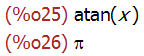
'limit(sin(x)/x,x,0);
limit(sin(x)/x,x,0);
'limit((1+1/x)^x,x,inf);
limit((1+1/x)^x,x,inf);
limit((2^(1/x)+1)/(2^(1/x)-1),x,0);
'limit((2^(1/x)+1)/(2^(1/x)-1),x,0,minus);
limit((2^(1/x)+1)/(2^(1/x)-1),x,0,minus);
'limit((2^(1/x)+1)/(2^(1/x)-1),x,0,plus);
limit((2^(1/x)+1)/(2^(1/x)-1),x,0,plus);
'limit((2*x^2+x)/(x^2-2),x,inf);
limit((2*x^2+x)/(x^2-2),x,inf);

### 微分运算
diff 函数可以实现微分运算,有四种基本形式,最基本的形式是:
diff (expr, x) 求表达式 expr 对 x 的微分。
diff(sin(x)*x^3,x);
diff(u(x)*v(x),x);
diff(u(x)*v,x);
从上面的例子可以看到,一个函数如果不明确表明自变量,diff 函数是不会对其求导的。
diff (expr, x, n)
求表达式 expr 对 x 的 n 次微分。
diff(y^3*exp(-y^2),y,2);

diff (expr, x_1, n_1, …, x_m, n_m) 求的是混合偏导数。
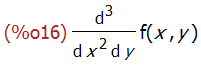
diff(f(x,y),x,2,y,1);
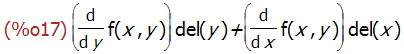
diff (expr) 计算的是全微分。
diff(f(x,y));
### taylor 级数展开
函数f(x)的在x = a附近的幂级数可以通过powerseries (f(x), x, a)获得。
powerseries (f(x), x, a);
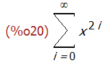
powerseries(1/(1-x^2), x, 0);
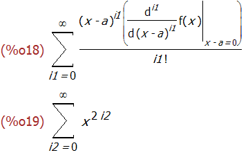
上面得到的结果中的求和指数 i2 看起来显得不那么专业,可以用 niceindices 函数将其变的看起来更专业些。
niceindices(powerseries(1/(1-x^2), x, 0));
很多时候我们无法得到级数的解析表示,这时候可以用 taylor (f(x), x, a, n)得到函数f(x)在x = a附近第 n 阶项((x - a)^n)以下各项的泰勒级数
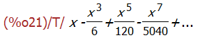
taylor(sin(x), x, 0, 8);
同样,对多元函数也可以进行 taylor 展开。
taylor (sin (y + x), x, 0, 3, y, 0, 3);

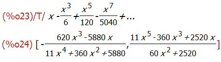
利用 pade 近似可以将 taylor 级数转化为多项式函数。比如下面的例子
taylor(sin(x), x, 0, 8);
pade(%,5,5);
### 积分运算
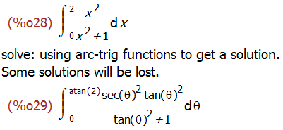
integrate(expr, x)
计算不定积分。
integrate(expr, x, a, b)
计算定积分,积分上下限分别为 a b。
integrate(1/(1+x^2),x);
integrate(1/(1+x^2),x, minf, inf);
risch (expr, x)
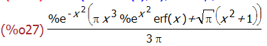
采用 Risch 方法计算不定积分。
risch (x^2*erf(x), x),ratsimp;
changevar 函数利用变量替换,对待积分函数进行换元。这个功能对学习换元法求积分还是蛮有用的。
'integrate(x^2/(1+x^2),x,0,2);
changevar(%,x=tan(theta),theta,x);
### 求和与求积运算
sum (expr, i, i_0, i_1)
计算求和。
product (expr, i, i_0, i_1)
计算求积。
sum (i^2, i, 1, 7);
sum (a[i], i, 1, 7);
sum(1/k^2,k,0,inf);
sum (1/3^i, i, 1, inf), simpsum;
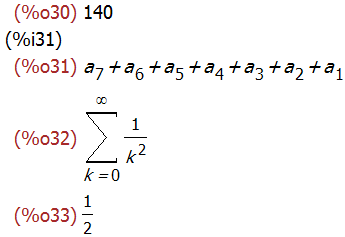
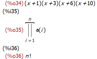
product (x + i*(i+1)/2, i, 1, 4);
product (a(i), i, 1, n);
product (k, k, 1, n), simpproduct;
### laplace 变换
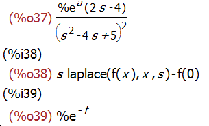
Maxima 中提供了两个函数用来计算 laplace 变换和反变换。
laplace (expr, t, s) 对表达式 expr 进行 laplace 变换,积分变量为 t,变换后的参数为 s.
ilt (expr, s, t) 对表达式进行反变换。
需要说明的是这两个函数进行的都是单边 laplace 变换,Maxima 中还没有对双边拉式变换的支持。
laplace (exp (2*t + a) * sin(t) * t, t, s);
laplace ('diff (f (x), x), x, s);
ilt(1/(s+1),s,t);
提到 laplace 变换就不能不提提部分分式展开。
在大多数介绍 laplace 变换的初级课本中都只介绍利用部分分式展开的方式进行反变换。
Maxima 提供了 partfrac 函数来完成部分分式展开的工作。下面用一个例子来说明:
x/(x^3+4*x^2+5*x+2);
partfrac (x/(x^3+4*x^2+5*x+2), x);

Maxima 的三角函数化简功能
最后更新于:2022-04-01 07:31:35
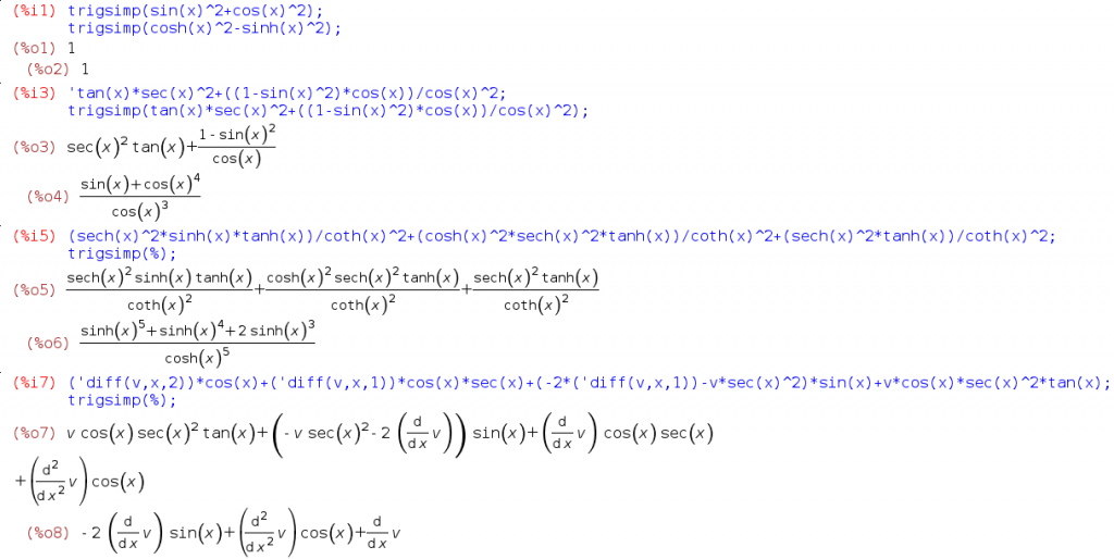
trigsimp 函数是最基本的用来对三角函数进行化简的功能函数。 trigsimp 函数利用 sin(x)^2 + cos(x)^2 = 1 and cosh(x)^2 - sinh(x)^2 = 1 来进行化简。
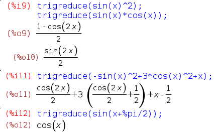
trigreduce 函数利用多倍角公式将三角函数的幂次转换为多倍角。
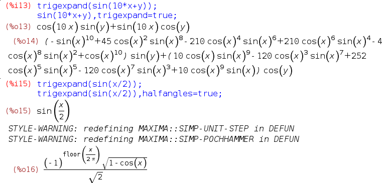
trigexpand 函数用来将三角函数展开。
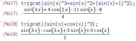
trigrat 函数将三角函数表达式展开为一种近似线性的形式。
Maxima 中的复数运算
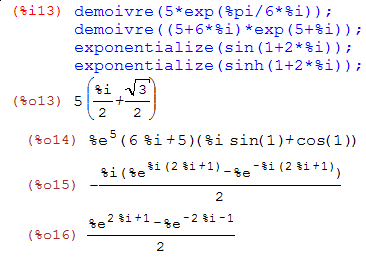
最后更新于:2022-04-01 07:31:31
在 Maxima 中用 %i 表示单位虚数。四则运算和大多数的函数直接就支持复数。比如下面的例子:

rectform 函数可以将输入的复数化为标准的直角坐标形式。
polarform 函数则将复数化为极坐标形式。

realpart 和 imagpart 函数分别提取函数的实部和虚部。

demoivre 函数利用 De Moivre 公式将带复数的指数函数化为三角函数形式。
exponentialize 函数利用 De Moivre 公式将带复数的三角函数化为指数函数形式。
carg 和 cabs 函数分别计算复数的辐角和模。conjugate 计算复数的共轭。

residue 函数可以用来计算留数(残数)。

maxima 代数方程求解
最后更新于:2022-04-01 07:31:29
本文最初写于 2010-07-21于 sohu 博客,这次博客搬家一起搬到这里来。
版权所有,转载请注明出处。
# 一般的代数方程
solve (expr, x)
solve (expr)
solve ([eqn_1, ..., eqn_n], [x_1, ..., x_n])
几个例子:
solve (asin (cos (3*x))*(f(x) - 1), x);

[4*x^2 - y^2 = 12, x*y - x = 2];
solve (%, [x, y]);

# 多项式方程
realroots 计算多项式方程的数值解.
realroots (expr, bound)
realroots (eqn, bound)
realroots (expr)
realroots (eqn)
几个例子:
realroots (-1 - x + x^5, 5e-6);
realroots (expand ((1 - x)^5 * (2 - x)^3 * (3 - x)), 1e-20);

allroots 计算多项式方程的全部解.
allroots (expr)
allroots (eqn)
几个例子:
eqn: (1 + 2*x)^3 = 13.5*(1 + x^5);
soln: allroots (eqn);

# 二分法求数值解
find_root (expr, x, a, b)
find_root (f, a, b)
几个例子:
find_root (sin(x) - x/2, x, 0.1, %pi);
find_root (sin(x) = x/2, x, 0.1, %pi);

f(x) := sin(x) - x/2;
find_root (f(x), x, 0.1, %pi);

# 牛顿迭代法
newton (expr, x, x_0, eps)
mnewton (FuncList,VarList,GuessList)
newton 用来解方程,mnewton 用来解方程组
几个例子:
load (newton1)$
newton (cos (u), u, 1, 1/100);

assume (a > 0);
newton (x^2 - a^2, x, a/2, a^2/100);

load("mnewton")$
mnewton([x1+3*log(x1)-x2^2, 2*x1^2-x1*x2-5*x1+1], [x1, x2], [5, 5]);

# 线性代数方程组
linsolve ([expr_1, ..., expr_m], [x_1, ..., x_n])
几个例子:
e1: x + z = y;
e2: 2*a*x - y = 2*a^2;
e3: y - 2*z = 2;
linsolve ([e1, e2, e3], [x, y, z]);

# 多项式方程组
algsys ([expr_1, ..., expr_m], [x_1, ..., x_n])
algsys ([eqn_1, ..., eqn_m], [x_1, ..., x_n])
几个例子:
e1: 2*x*(1 - a1) - 2*(x - 1)*a2;
e2: a2 - a1;

e3: a1*(-y - x^2 + 1);
e4: a2*(y - (x - 1)^2);
algsys ([e1, e2, e3, e4], [x, y, a1, a2]);
