13. COMPUTER GRAPHICS

## 13.1\. WHAT’S THE BIG PICTURE?[](http://csfieldguide.org.nz/ComputerGraphics.html#what-s-the-big-picture "Permalink to this headline") Computer graphics will be familiar from games, films and images, and there is amazing software available to create images, but how does the software work? The role of a computer scientist is not just to *use* graphics systems, but to *create* them, and especially invent new techniques. The entertainment industry is always trying to develop new graphics software so that they can push the boundaries and create new experiences. We’ve seen this in the evolution of animated films, from simple 2D films to realistic computer generated movies with detailed 3D images. Movie and gaming companies can’t always just use existing software to make the next great thing — they need computer scientists to come up with better graphics techniques to make something that’s never been seen before. The creative possibilities are endless! Computer graphics are used in a wide variety of situations: games and animated movies are common examples, but graphics techniques are also used to visualise large amounts of data (such as all cellphone calls being made in one day), to display and animate graphical user interfaces, to create virtual reality and augmented reality worlds, and much more. In this chapter we’ll look at some of the basic techniques that are used to create computer graphics. These will give you an idea of the techniques that are used in graphics programming, although it’s just the beginning of what’s possible. For this chapter we are using a system called WebGL which can render 3D graphics in your browser. If your browser is set up correctly then you should see a teapot on the right, and you can click the “animate” button to make it rotate. If this doesn’t work, or if the performance is poor, there is [information here about how to get it going](http://csfieldguide.org.nz/appendices/Interactives.html) . ## 13.2\. GRAPHICS TRANSFORMS[](http://csfieldguide.org.nz/ComputerGraphics.html#graphics-transforms "Permalink to this headline") A computer graphics image is just the result of a whole lot of mathematical calculations. In fact, every pixel you see in an image has typically had many calculations made to work out what colour it should be, and there are often millions of pixels in a typical image. Let’s start with some simple but common calculations that are needed for in graphics programming. The following image shows a cube with writing on each face. You can move it around using what’s called a *transform*, which simply adjusts where it is placed in space. In this example the only transforms we've supplied are to *translate* it in three dimensions. The dimensions are *x* (left and right), *y* (up and down) and *z* (in and out of the screen). Your goal is to type in how far it should be transformed in each of these directions so that you can see the symbol on each face, and put those symbols on the spinner wheels shown. (The order of the symbols doesn't matter). [Click to load the widget](http://csfieldguide.org.nz/ComputerGraphics.html) You’ve just applied 3D *translation transforms* to the cube. Translation just means moving it in the three dimensions up and down, forward and back, and sideways. 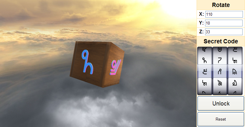Another common transform is *rotation*, which you can use in the following image to find the symbols (the rotation is measured in degrees). [Click to load the widget](http://csfieldguide.org.nz/ComputerGraphics.html) There are several transformations that are used in computer graphics, but the most common ones are translation (moving the object), rotation (spinning it) and scaling (changing its size). They come up often in graphics because they are applied not only to objects, but to things like the positions of the camera and lighting sources. In this section you can apply transformations to various images. We’ll start by making the changes manually, one point at a time, but we’ll move up to a quick shortcut method that uses a *matrix* to do the work for you. We’ll start by looking at how these work in two dimensions - it’s a bit easier to think about than three dimensions. 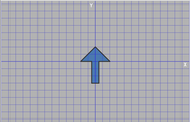The following interactive shows an arrow, and on the right you can see a list of the points that correspond to its 7 corners. The arrow is on a grid (usually referred to as *cartesian coordinates* ), where the centre point is the “zero” point. Points are specified using two numbers, *x* and *y*, usually written as (*x*,*y*). The *x* value is how far the point is to the right of the centre and the *y* value is how far above the centre it is. For example, the first point in the list is the tip at (0,2), which means it’s 0 units to the right of the centre (i.e. at the centre), and 2 units above it. Which point does the last pair (2,0) correspond to? What does it mean if a coordinate has a negative*x* value? The first list of coordinates is for the original arrow position, and in the second list, you can type in the transformed points to move the arrow — the original is shown in green and the moved one is in blue. [Click to load the widget](http://csfieldguide.org.nz/ComputerGraphics.html) Your first challenge is to add 2 to all the *x* points, and 3 to all the *y* points (you can either type the new number or put the calculation in the box e.g. "0.5+2". What effect does this have on the original arrow? (Be careful to add the negative numbers correctly; for example, adding 2 to -0.5 gives 1.5.) What happens if you subtract 3 from each of the original coordinate values? The above transform is called a *translation* — it translates the arrow around the grid. This kind of transform is used in graphics to specify where an object should be placed in a scene, but it has many other uses, such as making an animated object move along a path, or specifying the position of the imaginary camera (viewpoint). 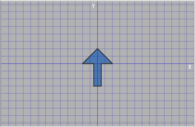In this next interactive, try replacing the coordinates in the second list with all the original values multiplied by 2\. What is the effect of this transform? What would happen if you multiply each value by 10? How about 0.5? What if you only multiply the *x* values? [Click to load the widget](http://csfieldguide.org.nz/ComputerGraphics.html) This transformation is called *scaling*, and although it can obviously be used to control the size of an object, this can in turn be used to create a visual effect such as making the object appear closer or further away. 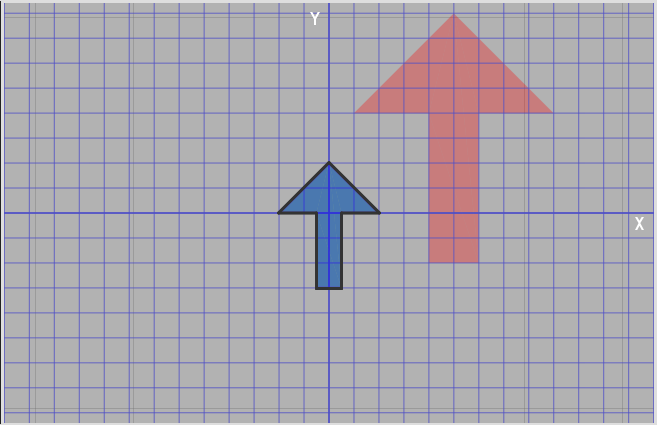Try to get the blue arrow to match up with the red one. It will require a mixture of scaling and translation. 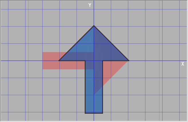[Click to load the widget](http://csfieldguide.org.nz/ComputerGraphics.html) Next, see what happens if you swap the *x* and *y* value for each coordinate. [Click to load the widget](http://csfieldguide.org.nz/ComputerGraphics.html) This is a simple *rotation* transformation, also useful for positioning objects in a scene, but also for specifying things like camera angles. ### 13.2.1\. MATRIX TRANSFORMS[](http://csfieldguide.org.nz/ComputerGraphics.html#matrix-transforms "Permalink to this headline") There’s a much easier way to specify transformations than having to change each coordinate separately. Transformations are usually done in graphics using *matrix*arithmetic, which is a shorthand notation for doing lots of simple arithmetic operations in one go. The matrix for the two-dimensional transformations we’ve been doing above has four values in it. For the 2 dimensional scaling transform where we made each *x* and *y* value twice as large, the matrix is written as: [2002] You can type this matrix into the following interactive to see what it does (replace the ones with twos). The top left-hand value just means multiply all the *x* values by 2, and the bottom right one means multiply all the *y* values by 2\. For the meantime, leave the other two values as 0. [ Click to load the widget.](http://csfieldguide.org.nz/ComputerGraphics.html) (At this stage you may want to have the widget open in a separate window so that you can read the text below and interact with the widget at the same time.) Now try changing the matrix to [3003] or [0.2000.2] The “add translate” values in the interactive are added to each *x* and *y* coordinate; experiment with them to see what they do. Now try to find suitable values for these and the matrix to match the arrow up with the red one. What happens if you use the following matrix? [2004] Now try the following matrix: [0110] This matrix should have rotated the arrow to the right. A simple way of looking at the matrix is that the top row determines the transformed *x* value, simply by saying how much of the original *x* value and *y* value contribute to the new *x* value. So in the matrix: [2004] the top row just means that the new *x* value is 2 lots of the original *x*, and none of the original y, which is why all the *x* values double. The second row determines the *y*value: in the above example, it means that the new *y* value uses none of the original x, but 4 times the original *y* value. If you try this matrix, you should find that the location of all the *x* points is doubled, and the location of all the y points is multiplied by 4. That now explains the [0110] matrix. The new *x* value has none of the original *x*, but exactly the original *y* value, and vice versa. This swaps all the *x* and *y*coordinates, which is the same as rotating the object to the right. Where it gets interesting is when you use a little of each value; try the following matrix: [0.7−0.70.70.7] Now the *x* value of each coordinate is a mixture of 0.7 of the original *x*, and 0.7 of the original *y*. 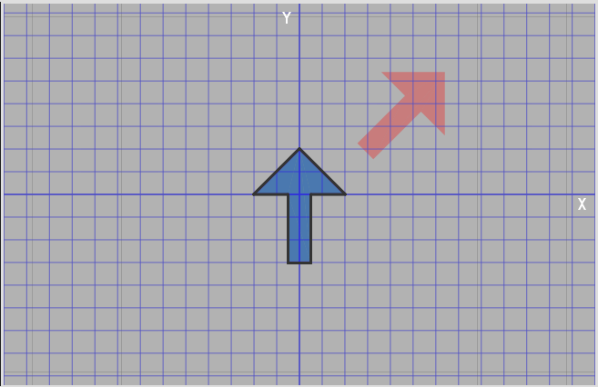In general, to rotate an image by a given angle you need to use the sine (abbreviated sin) and cosine (abbreviated cos) functions from trigonometry. To rotate the image by Θ degrees, you’ll need the following values in the matrix, which rely on trig functions: [cos(θ)sin(θ)−sin(θ)cos(θ)] You can type these calculations directly into the interactive - if you type cos(60) it will work out the cosine of 60 degrees for you, which happens to be exactly 0.5\. Or you can just type in the sin and cosine values; the 0.7 numbers in the matrix above are just the values for sin(45) and so on (or at least, they approximately the value; it's actually 0.70710678..., which happens to be the square root of 0.5, but 0.7 is close enough for our example). [ Click to load the widget.](http://csfieldguide.org.nz/ComputerGraphics.html) What is the matrix for rotation by 360 degrees? 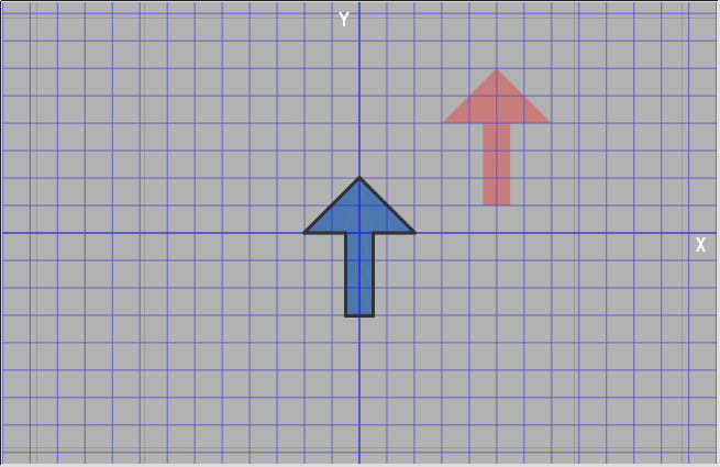The general matrix for *scaling* is a bit simpler; if you want to scale by a factor of *s*, then you just use the matrix: [s00s] A translation can’t be specified by this kind of matrix, but in the interactives we’ve provided an extra place to specify an *x* and *y* value to translate the input. Try translating the original arrow so that it matches up with the red arrow. [ Click to load the widget.](http://csfieldguide.org.nz/ComputerGraphics.html) Now try to scale the original arrow in the following, and translate it to match the red arrow. 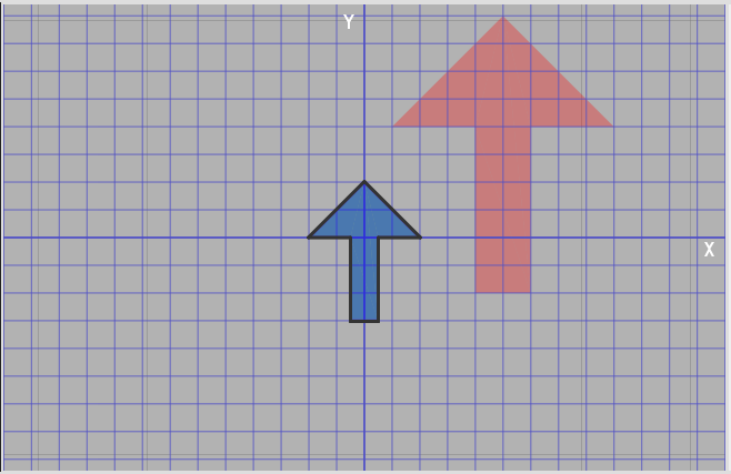[ Click to load the widget.](http://csfieldguide.org.nz/ComputerGraphics.html) The following interactive has the translation and scaling the other way around. Use this one to transform the blue arrow to the red arrow. The order in which the operations happen makes a difference! 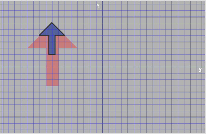[ Click to load the widget.](http://csfieldguide.org.nz/ComputerGraphics.html) In the above, you’ll have noticed that scaling is affected by how far the object is from the centre. If you want to scale around a fixed point in the object (so it expands where it is), then an easy way is to translate it back to the centre (also called the *origin*), scale it, and then translate it back to where it was. The following interactive allows you to move the arrow, then scale it, and move it back. The tip is at (-8,7), so you should translate it to (0,0), scale by 2, and translate back to (-8, 7). 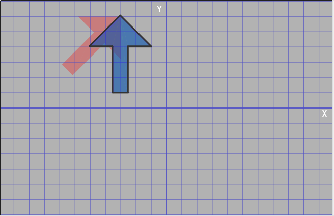[ Click to load the widget.](http://csfieldguide.org.nz/ComputerGraphics.html) The same problem comes up with rotation. Try rotating this image by 45 degrees.You'll need to translate the tip to the origin, apply the rotation, and translate it back. 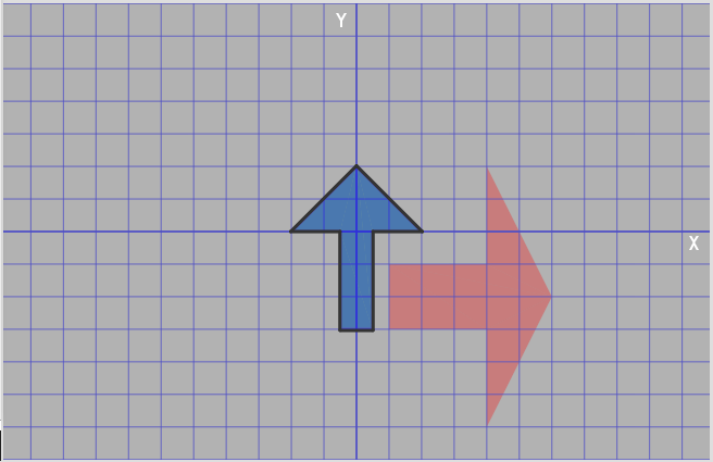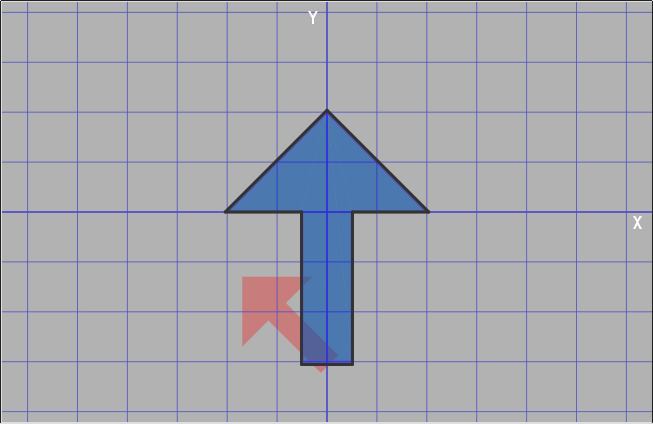[ Click to load the widget.](http://csfieldguide.org.nz/ComputerGraphics.html) The following two examples combine rotation, scaling and translation. You can use multiple matrices (that’s the plural of matrix) to match up the target object — the product of each matrix becomes the input to the next one. Oh, and the arrow is twice as fat, but still the same hight (from base to tip). Try matching the blue arrow to the red one using two matrices (one to scale and one to rotate), and adding a vector. [ Click to load the widget.](http://csfieldguide.org.nz/ComputerGraphics.html) You will need to use all three operations to do this next one. [ Click to load the widget.](http://csfieldguide.org.nz/ComputerGraphics.html) These combined transformations are common, and they might seem like a lot of work because each matrix has to be applied to every point in an object. Our arrows only had 7 points, but complex images can have thousands or even millions of points in them. Fortunately we can combine all the matrix operations in advance to give just one operation to apply to each point. ### 13.2.2\. COMBINING TRANSFORMATIONS[](http://csfieldguide.org.nz/ComputerGraphics.html#combining-transformations "Permalink to this headline") Several transforms being applied to the same image can be made more efficient by creating one matrix that has the effect of all the transforms combined.The combination is done by “multiplying” all the matrices. Multiplying two matrices can’t be done by just multiplying the corresponding elements; if you are multiplying two matrices with the *a* and *b* values shown below, the resulting values from the multiplication are calculated as follows: [a11a12a21a22] \times [b11b12b21b22] = [a11b11+a21b12a12b11+a22b12a11b21+a21b22a12b21+a22b22] It’s a bit complicated, but this calculation is only done once to work out the combined transformation, and it gives you a single matrix that will provide to transforms in one operations. As a simple example, consider what happens when you scale by 2 and then rotate by 45 degrees. The two matrices to multiply work out like this: [2002] \times [0.7−0.70.70.7] = [2×0.7+0×−0.70×0.7+2×−0.72×0.7+0×0.70×0.7+2×0.7] = [1.4−1.41.41.4] Try putting in the final matrix here and see if it does scale by 2 and rotate by 45 degrees. [ Click to load the widget.](http://csfieldguide.org.nz/ComputerGraphics.html) Now try multiplying two other transform matrices that you make up yourself, and see if they produce the expected result. [ Click to load the widget.](http://csfieldguide.org.nz/ComputerGraphics.html) In computer graphics systems there can be many transformations combined, and this is done by multiplying them all together (two at a time) to produce one matrix that does all the transforms in one go. That transform might then be applied to millions of points, so the time taken to do the matrix multiplication at the start will pay off well. The project below gives the chance to explore combining matrices, and has an interactive that will calculate the multiplied matrices for you. ### 13.2.3\. 3D TRANSFORMS[](http://csfieldguide.org.nz/ComputerGraphics.html#d-transforms "Permalink to this headline") So far we’ve just done the transforms in two dimensions. To do this in 3D, we need a *z* coordinate as well, which is the depth of the object into the screen. A matrix for operating on 3D points is 3 by 3\. For example, the 3D matrix for doubling the size of an object is as follows; it multiplies each of the *x*, *y* and *z* values of a point by 2. ⎡⎣⎢200020002⎤⎦⎥ In this interactive, try changing the scaling on the image (it starts with a scaling factor of 10 in all three dimensions). [ Click to load the widget.](http://csfieldguide.org.nz/ComputerGraphics.html) The above image mesh has 3644 points in it, and your matrix was applied to each one of them to work out the new image. Translation requires 3 values, which are added to the *x*, *y* and *z* coordinates of each point in an object. In the following interactive, try moving the teapot left and right ( *x* ), up and down ( *y* ), and in and out of the screen ( *z* ) by adding a “vector” to the operations. Then try combining all three. [ Click to load the widget.](http://csfieldguide.org.nz/ComputerGraphics.html) Rotation is trickier because you can now rotate in different directions. In 2D rotations were around the centre (origin) of the grid, but in 3D rotations are around a line (either the horizontal x-axis, the vertical y-axis, or the z-axis, which goes into the screen!) The rotation we used earlier can be applied to 3 dimensions using this matrix: ⎡⎣⎢cos(θ)sin(θ)0−sin(θ)cos(θ)0001⎤⎦⎥ Try applying that to the image above. This is rotating around the z-axis (a line going into the screen); that is, it’s just moving the image around in the 2D plane. It’s really the same as the rotation we used previously, as the last line (0, 0, 1) just keeps the z point the same. Try the following matrix, which rotates around the x-axis (notice that the x value always stays the same because of the 1,0,0 in the first line): ⎡⎣⎢1000cos(θ)sin(θ)0−sin(θ)cos(θ)⎤⎦⎥ And this one for the y-axis: ⎡⎣⎢cos(θ)0−sin(θ)010sin(θ)0cos(θ)⎤⎦⎥ The following interactive allows you to combine 3D matrices. You can experiment with moving the teapot around in space, changing its size, and angle. Think about the order in which you need to combine the transforms to get a particular image that you want. For example, if you translate an image and then scale it, you’ll get a different effect to scaling it then translating it. If you want to rotate or scale around a particular point, you can do this in three steps (as with the 2D case above): (1) translate the object so that the point you want to scale or rotate around is the origin (where the x, y and z axes meet), (2) do the scaling/rotation, (3) translate the object back to where it was. If you just scale an object where it is, its distance from the origin will also be scaled up. 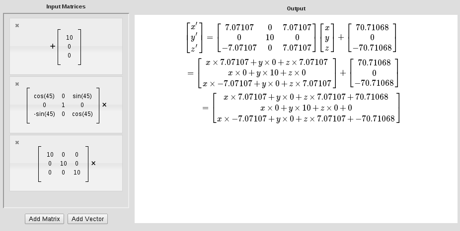[ Click here for the interactive to combine multiple transforms into one](http://csfieldguide.org.nz/ComputerGraphics.html) In the above examples, when you have several matrices being applied to every point in the image, a lot of time can be saved by converting the series of matrices and transforms to just one formula that does all of the transforms in one go. The following interactive can do those calculations for you. For example, in the following interactive, type in the matrix for doubling the size of an object (put the number 2 instead of 1 on the main diagonal values), then add another matrix that triples the size of the image (3 on the main diagonal). The interactive shows a matrix on the right that combines the two — does it look right? Multiple transforms [ Click to load the widget.](http://csfieldguide.org.nz/ComputerGraphics.html) The interactive also allows you to combine in translations (just three numbers, for x, y and z). Try combining a scaling followed by a translation. What if you add a rotation — does the order matter? In case you’re wondering, the interactive is using the following formula to combine two matrices (you don’t have to understand this to use it). It is called matrix multiplication, and while it might be a bit tricky, it’s very useful in computer graphics because it reduces all the transformations you need to just one matrix, which is then applied to every point being transformed. This is way better than having to run all the matrices of every point. ### 13.2.4\. PROJECT: 3D TRANSFORMS[](http://csfieldguide.org.nz/ComputerGraphics.html#project-3d-transforms "Permalink to this headline") For this project, you will demonstrate what you’ve learned in the section above by explaining a 3D transformation of a few objects. You should take screenshots of each step to illustrate the process for your report. The following scene-creation interactive allows you to choose objects (and their colours etc.), and apply one transformation to them. To position them more interestingly, you will need to come up with multiple transformations (e.g. scale, then rotate, then translate), and use the “simplifier” interactive to combine all the matrices into one operation. The scene-creation interactive can be run from here: [ Click to load the widget.](http://csfieldguide.org.nz/ComputerGraphics.html) To generate combined transformations, you can use the following transform simplifier interactive: [ Click to load the widget.](http://csfieldguide.org.nz/ComputerGraphics.html) Because you can’t save your work in the interactives, keep notes and screen shots as you go along. These will be useful for your report, and also can be used if you need to start over again. Introduce your project with a examples of 3D images, and how they are used (perhaps from movies or scenes that other people have created). Describe any innovations in the particular image (e.g. computer generated movies usually push the boundaries of what was previously possible, so discuss what boundaries were moved by a particular movie, and who wrote the programs to achieve the new effects). For your project, try putting a few objects in a particular arrangement (e.g. with the teapot sitting beside some cups), and explain the transforms needed to achieve this, showing the matrices needed. Give simple examples of translation, scaling *and* rotation using your scene. You should include multiple transforms applied to one object, and show how they can be used to position an object. Show how the matrices for a series of transforms can be multiplied together to get one matrix that applies all the transforms at once. Discuss how the single matrix derived from all the others is more efficient, using your scene as an example to explain this. ## 13.3\. DRAWING LINES AND CIRCLES[](http://csfieldguide.org.nz/ComputerGraphics.html#drawing-lines-and-circles "Permalink to this headline") A fundamental operation is computer graphics is to draw lines and circles. For example, these are used as the components of scalable fonts and vector graphics; the letter “i” is specified as a series of lines and curves, so that when you zoom in on it the computer can redraw it at whatever resolution is needed.  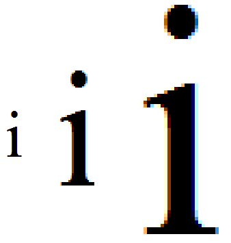In 3D graphics shapes are often stored using lines and curves that mark out the edges of flat surfaces, each of which is so small that you can’t see them unless you zoom right in.  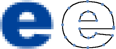The lines and circles that specify an object are usually given using numbers (for example, a line between a given starting and finishing position or a circle with a given centre and radius). From this a graphics program must calculate which pixels on the screen should be coloured in to represent the line or circle. 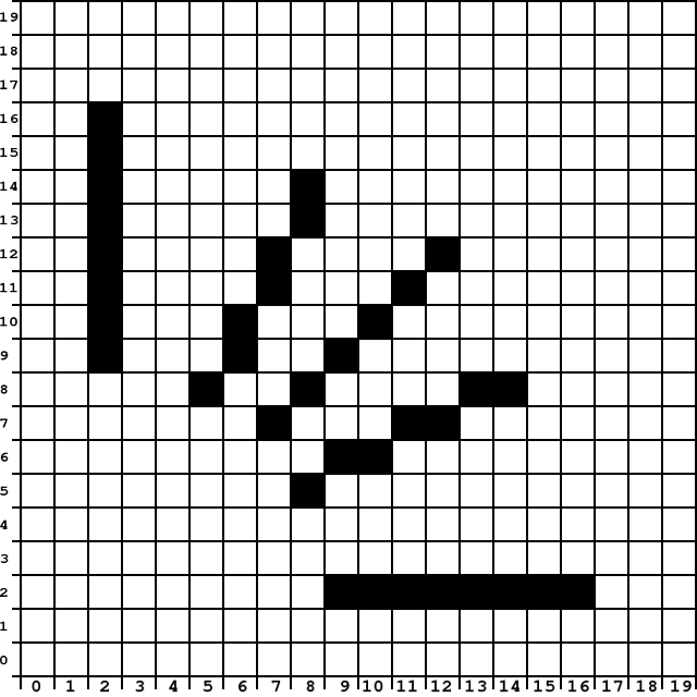For example, here’s a grid of pixels with 5 lines shown magnified. The vertical line would have been specified as going from pixel (2,9) to (2,16) — that is, starting 2 across and 9 up, and finishing 2 across and 16 up. Of course, this is only a small part of a screen, as normally they are more like 1000 by 1000 pixels or more; even a smartphone can be hundreds of pixels high and wide. [](http://csfieldguide.org.nz/_images/20grid_example.png) These are things that are easy to do with pencil and paper using a ruler and compass, but on a computer the calculations need to be done for every pixel, and if you use the wrong method then it will take too long and the image will be displayed slowly or a live animation will appear jerky. In this section we will look into some very simple but clever algorithms that enable a computer to do these calculations very quickly. ### 13.3.1\. 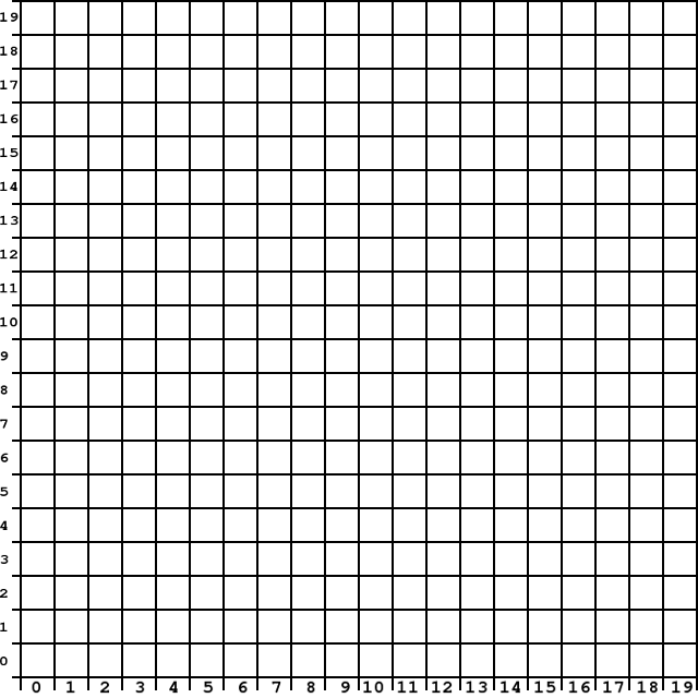LINE DRAWING[](http://csfieldguide.org.nz/ComputerGraphics.html#line-drawing "Permalink to this headline") To draw a line, a computer must work out which pixels need to be filled so that the line looks straight. You can try this by colouring in squares on a grid, such as the one below (they are many times bigger than the pixels on a normal printer or screen). We’ll identify the pixels on the grid using two values, (*x*,*y*), where *x* is the distance across from the left, and *y* is the distance up from the bottom. The bottom left pixel below is (0,0), and the top right one is (19,19). On the following grid, try to draw these straight lines by filling in pixels in the grid: * from (2, 17) to (10, 17) * from (18, 2) to (18, 14) * from (1, 5) to (8, 12) [](http://csfieldguide.org.nz/_images/20grid.png) Drawing a horizontal, vertical or diagonal line like the ones above is easy; it’s the ones at different angles that require some calculation. Without using a ruler, can you draw a straight line from A to B on the following grid by colouring in pixels? [](http://csfieldguide.org.nz/_images/20grid_ab.png) Once you have finished drawing your line, try checking it with a ruler. Place the ruler so that it goes from the centre of A to the centre of B. Does it cross all of the pixels that you have coloured? ### 13.3.2\. USING A FORMULA TO DRAW A LINE[](http://csfieldguide.org.nz/ComputerGraphics.html#using-a-formula-to-draw-a-line "Permalink to this headline") The mathematical formula for a line is y=mx+c. This gives you the *y* value for each *x* value across the screen, where m is the slope of the line and c is where it crosses the y axis. In other words, for *x* pixels across, the pixel to colour in would be (*x*, mx+c). For example, choosing m=2 and c=3 means that the line would go through the points (0,3), (1,5), (2,7), (3,9) and so on. This line goes up 2 pixels for every one across (m=2), and crosses the y axis 3 pixels up (c=3). You should experiment with drawing graphs for various values of m and c (for example, start with c=0, and try these three lines: m=1, m=0.5 and m=0) by putting in the values. What angle are these lines at? The mx+c formula can be used to work out which pixels should be coloured in for a line that goes between (x1,y1) and (x2,y2). What are (x1,y1) and (x2,y2) for the points A and B on the grid below? See if you can work out the m and b values for a line from A to B, or you can calculate them using the following formulas: m=(y2−y1)(x2−x1) b=(y1x2−y2x1)(x2−x1) Now draw the same line as in the previous section (between A and B) using the formula y=mx+c to calculate *y* for each value of *x* from x1 to x2 (you will need to round *y* to the nearest integer to work out which pixel to colour in). If the formulas have been applied correctly, the *y* value should range from y1 to y2. [](http://csfieldguide.org.nz/_images/20grid_ab.png) Once you have completed the line, check it with a ruler. How does it compare to your first attempt? Now consider the number of calculations that are needed to work out each point. It won’t seem like many, but remember that a computer might be calculating hundreds of points on thousands of lines in a complicated image. In the next section we will explore a method that greatly speeds this up. ### 13.3.3\. BRESENHAM’S LINE ALGORITHM[](http://csfieldguide.org.nz/ComputerGraphics.html#bresenham-s-line-algorithm "Permalink to this headline") A faster way for a computer to calculate which pixels to colour in is to use Brensenham’s Line Algorithm. It follows these simple rules. First, calculate these three values: A=2×(y2−y1) B=A−2×(x2−x1) P=A−(x2−x1) To draw the line, fill the starting pixel, and then for every position along the *x* axis: * if P is less than 0, draw the new pixel on the same line as the last pixel, and add A to P. * if P was 0 or greater, draw the new pixel one line higher than the last pixel, and add B to P. * repeat this decision until we reach the end of the line. Without using a ruler, use Bresenham’s Line Algorithm to draw a straight line from A to B: [](http://csfieldguide.org.nz/_images/20grid_ab.png) Once you have completed the line, check it with a ruler. How does it compare to the previous attempts? ### 13.3.4\. LINES AT OTHER ANGLES[](http://csfieldguide.org.nz/ComputerGraphics.html#lines-at-other-angles "Permalink to this headline") So far the version of Bresenham’s line drawing algorithm that you have used only works for lines that have a gradient (slope) between 0 and 1 (that is, from horizontal to 45 degrees). To make this algorithm more general, so that it can be used to draw any line, some additional rules are needed: * If a line is sloping downward instead of sloping upward, then when P is 0 or greater, draw the next column’s pixel one row *below* the previous pixel, instead of above it. * If the change in Y value is greater than the change in X value, then the calculations for A, B, and the initial value for P will need to be changed. When calculating A, B, and the initial P, use X where you previously would have used Y, and vice versa. When drawing pixels, instead of going across every column in the X axis, go through every row in the Y axis, drawing one pixel per row. [](http://csfieldguide.org.nz/_images/20grid.png) In the grid above, choose two points of your own that are unique to you. Don’t choose points that will give horizontal, vertical or diagonal lines! Now use Bresenham’s algorithm to draw the line. Check that it gives the same points as you would have chosen using a ruler, or using the formula y=mx+b. How many arithmetic calculations (multiplications and additions) were needed for Bresenhams algorithm? How many would have been needed if you used the y=mx+b formula? Which is faster (bear in mind that adding is a lot faster than multiplying for most computers). You could write a program or design a spreadsheet to do these calculations for you — that’s what graphics programmers have to do. ### 13.3.5\. CIRCLES[](http://csfieldguide.org.nz/ComputerGraphics.html#circles "Permalink to this headline") As well as straight lines, another common shape that computers often need to draw are circles. An algorithm similar to Bresenham’s line drawing algorithm, called the Midpoint Circle Algorithm, has been developed for drawing a circle efficiently. A circle is defined by a centre point, and a radius. Points on a circle are all the radius distance from the centre of the circle. 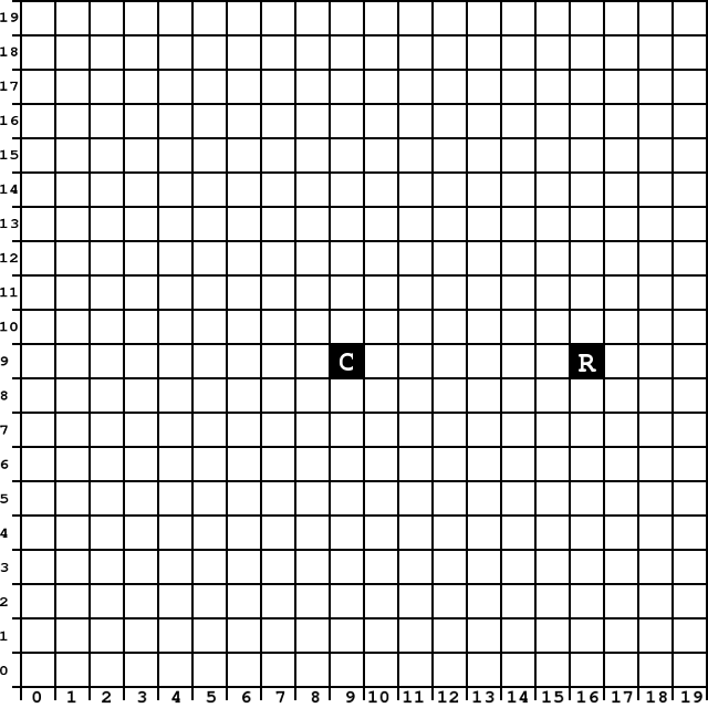[](http://csfieldguide.org.nz/_images/20grid_cr.png) Try to draw a circle by hand by filling in pixels (without using a ruler or compass). Note how difficult it is to make the circle look round. It is possible to draw the circle using a formula based on Pythagoras’ theorem, but it requires calculating a square root for each pixel, which is very slow. The following algorithm is much faster, and only involves simple arithmetic so it runs quickly on a computer. ### 13.3.6\. BRESENHAM’S MIDPOINT CIRCLE ALGORITHM[](http://csfieldguide.org.nz/ComputerGraphics.html#bresenham-s-midpoint-circle-algorithm "Permalink to this headline") Here are the rules for the Midpoint Circle Algorithm for a circle around (cx, cy) with a radius of R: E=−R X=R Y=0 Repeat the following rules in order until *Y* becomes greater than *X*: * Fill the pixel at coordinate (cx+X, cy+Y) * Increase *E* by 2×Y+1 * Increase *Y* by 1 * If *E* is greater than or equal to 0, subtract (2X−1) from *E*, and then subtract 1 from *X*. Follow the rules to draw a circle on the grid, using (cx, cy) as the centre of the circle, and R the radius. Notice that it will only draw the start of the circle and then it stops because *Y* is greater than *X*! [](http://csfieldguide.org.nz/_images/20grid_cr.png) When *y* becomes greater than *x*, one eighth (an octant) of the circle is drawn. The remainder of the circle can be drawn by reflecting the octant that you already have (you can think of this as repeating the pattern of steps you just did in reverse). Reflect pixels along the X and Y axis, such that the line of reflection crosses the middle of the centre pixel of the circle. Half of the circle is now drawn, the left and the right half. To add the remainder of the circle, another line of reflection must be used. Can you work out which line of reflection is needed to complete the circle? **Jargon Buster** : Octant A quadrant is a quarter of an area; the four quadrants that cover the whole area are marked off by a vertical and horizontal line that cross. An *octant* is one eighth of an area, and the 8 octants are marked off by 4 lines that intersect at one point (vertical, horizontal, and two diagonal lines). To complete the circle, you need to reflect along the diagonal. The line of reflection should have a gradient of 1 or -1, and should cross through the middle of the centre pixel of the circle. While using a line of reflection on the octant is easier for a human to understand, a computer can draw all of the reflected points at the same time it draws a point in the first octant because when it is drawing pixel with an offset of (x,y) from the centre of the circle, it can also draw the pixels with offsets (x,-y), (-x,y), (-x,-y), (y,x), (y,-x), (-y,x) and (-y,-x), which give all eight reflections of the original point! By the way, this kind of algorithm can be adapted to draw ellipses, but it has to draw a whole quadrant because you don’t have octant symmetry in an ellipse. ### 13.3.7\. PRACTICAL APPLICATIONS[](http://csfieldguide.org.nz/ComputerGraphics.html#practical-applications "Permalink to this headline") Computers need to draw lines, circles and ellipses for a wide variety of tasks, from game graphics to lines in an architect’s drawing, and even a tiny circle for the dot on the top of the letter ‘i’ in a word processor. By combining line and circle drawing with techniques like ‘filling’ and ‘antialiasing’, computers can draw smooth, clear images that are resolution independent. When an image on a computer is described as an outline with fill colours it is called vector graphics — these can be re-drawn at any resolution. This means that with a vector image, zooming in to the image will not cause the pixelation seen when zooming in to bitmap graphics, which only store the pixels and therefore make the pixels larger when you zoom in. However, with vector graphics the pixels are recalculated every time the image is redrawn, and that’s why it’s important to use a fast algorithm like the one above to draw the images. Outline fonts are one of the most common uses for vector graphics as they allow the text size to be increased to very large sizes, with no loss of quality to the letter shapes. Computer scientists have found fast algorithms for drawing other shapes too, which means that the image appears quickly and it can be done on relatively slow hardware - for example, a smartphone needs to do these calculations all the time to display images, and reducing the amount of calculations can extend its battery life, as well as make it appear faster. As usual, things aren’t quite as simple as shown here. For example, consider a horizontal line that goes from (0,0) to (10,0), which has 11 pixels. Now compare it with a 45 degree line that goes from (0,0) to (10,10). It still has 11 pixels, but the line is longer (about 41% longer to be precise). This means that the line would appear thinner or fainter on a screen, and extra work needs to be done (mainly anti-aliasing) to make the line look ok. We’ve only just begun to explore how techniques in graphics are needed to quickly render high quality images. ### 13.3.8\. PROJECT: LINE AND CIRCLE DRAWING[](http://csfieldguide.org.nz/ComputerGraphics.html#project-line-and-circle-drawing "Permalink to this headline") To compare Bresenham’s method with using the equation of a line (y=mx+b), choose your own start and end point of a line (of course, make sure it’s at an interesting angle), and show the calculations that would be made by each method. Count up the number of additions, subtractions, multiplications and divisions that are made in each case to make the comparison. Note that addition and subtraction is usually a lot faster than multiplication and division. You can estimate how long each operation takes on your computer by running a program that does thousands of each operation, and timing how long it takes for each. From this you can estimate the total time taken by each of the two methods. A good measurement for these is how many lines (of your chosen length) your computer could calculate per second. ## 13.4\. THE WHOLE STORY! ## 13.5\. FURTHER READING[](http://csfieldguide.org.nz/ComputerGraphics.html#further-reading "Permalink to this headline") Todo this section is yet to be written ### 13.5.1\. USEFUL LINKS[](http://csfieldguide.org.nz/ComputerGraphics.html#useful-links "Permalink to this headline") * [http://en.wikipedia.org/wiki/Computer_graphics](http://en.wikipedia.org/wiki/Computer_graphics) * [http://en.wikipedia.org/wiki/Transformation_matrix](http://en.wikipedia.org/wiki/Transformation_matrix) * [http://en.wikipedia.org/wiki/Bresenham](http://en.wikipedia.org/wiki/Bresenham)’s_line_algorithm * [http://en.wikipedia.org/wiki/Ray_trace](http://en.wikipedia.org/wiki/Ray_trace) * [http://www.cosc.canterbury.ac.nz/mukundan/cogr/applcogr.html](http://www.cosc.canterbury.ac.nz/mukundan/cogr/applcogr.html) * [http://www.cosc.canterbury.ac.nz/mukundan/covn/applcovn.html](http://www.cosc.canterbury.ac.nz/mukundan/covn/applcovn.html) * [http://www.povray.org/resources/links/3D_Tutorials/POV-Ray_Tutorials/](http://www.povray.org/resources/links/3D_Tutorials/POV-Ray_Tutorials/) Computer Graphics, Computer Vision, Bresenham’s Line Algorithm, Ray Tracing, Magnetic Resonance Imaging (MRI), Rendering, 3D Modeling, Animation, WebGL (Web Graphics Library), OpenGL (Open Graphics Library) ### 13.5.2\. KEY CONCEPTS[](http://csfieldguide.org.nz/ComputerGraphics.html#key-concepts "Permalink to this headline") * Algorithms: Bresenham’s algorithm (line and circle drawing), colour space conversion, line anti-aliasing, Bézier and B-spline curves, painter’s algorithm, Z-buffer * Techniques: Techniques: ray tracing, texture mapping, shading, anti-aliasing, volume rendering, polygonisation, constructive solid geometry, 3D modeling, hidden object removal * Applications: drawing software, animation